We evaluate the prediction accuracy of some simple models for the sunspots dataset.
import numpy as np
import pandas as pd
import matplotlib.pyplot as plt
import statsmodels.api as sm
sunspots = pd.read_csv('SN_y_tot_V2.0.csv', header = None, sep = ';')
print(sunspots.head())
y = sunspots.iloc[:, 1].values
n = len(y)
plt.figure(figsize = (12, 6))
plt.plot(y)
plt.show()
print(n) 0 1 2 3 4
0 1700.5 8.3 -1.0 -1 1
1 1701.5 18.3 -1.0 -1 1
2 1702.5 26.7 -1.0 -1 1
3 1703.5 38.3 -1.0 -1 1
4 1704.5 60.0 -1.0 -1 1
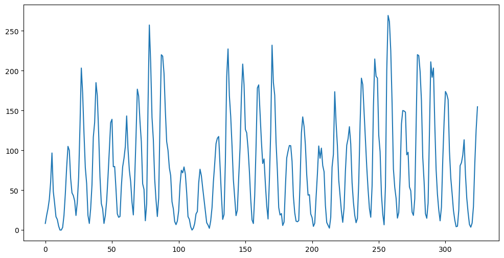
325
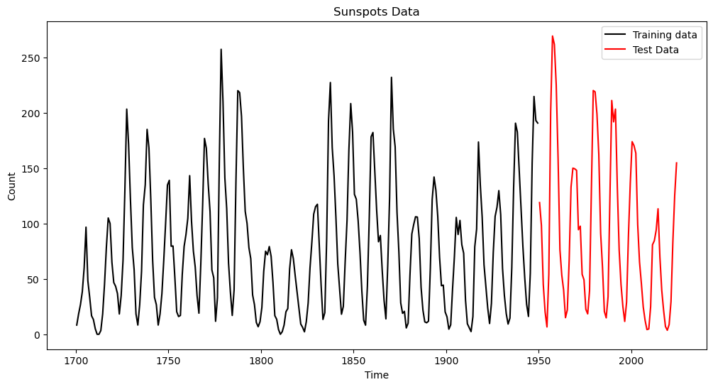
Let us split the dataset into two parts (training and test). We will fit models to the training data, and evaluate their prediction accuracy on the test set.
splitnumber = 250
sunspots_train = sunspots.iloc[:splitnumber, :].copy()
sunspots_test = sunspots.iloc[splitnumber:, :].copy()

print(sunspots_train)
print(sunspots_test)

tme_train = sunspots_train.iloc[:,0]
tme_test = sunspots_test.iloc[:,0]
tme = sunspots.iloc[:,0]

y =  sunspots_train.iloc[:,1].values

plt.figure(figsize = (12, 6))
plt.xlabel('Time')
plt.ylabel('Count')
plt.plot(tme, sunspots.iloc[:,1], color = "None")
plt.plot(tme_train, y, color = 'black', label = 'Training data')
plt.plot(tme_test, sunspots_test.iloc[:,1], color = 'red', label = 'Test Data')
plt.legend()
plt.title('Sunspots Data')
plt.show()
0 1 2 3 4
0 1700.5 8.3 -1.0 -1 1
1 1701.5 18.3 -1.0 -1 1
2 1702.5 26.7 -1.0 -1 1
3 1703.5 38.3 -1.0 -1 1
4 1704.5 60.0 -1.0 -1 1
.. ... ... ... ... ..
245 1945.5 55.3 6.6 365 1
246 1946.5 154.3 11.1 365 1
247 1947.5 214.7 9.8 365 1
248 1948.5 193.0 9.3 366 1
249 1949.5 190.7 9.2 365 1
[250 rows x 5 columns]
0 1 2 3 4
250 1950.5 118.9 7.3 365 1
251 1951.5 98.3 6.6 365 1
252 1952.5 45.0 4.5 366 1
253 1953.5 20.1 3.0 365 1
254 1954.5 6.6 1.7 365 1
.. ... ... ... ... ..
320 2020.5 8.8 4.1 14440 1
321 2021.5 29.6 7.9 15233 1
322 2022.5 83.2 14.2 15258 1
323 2023.5 125.5 19.2 13286 1
324 2024.5 154.7 22.1 11952 0
[75 rows x 5 columns]
Model One: Sinusoid Model
Our first model is the simple sinusoidal model that we studied way back in Lectures 5-8:
with . The point estimate for can be obtained by the follwoing code
def rss(f):
    n = len(y)
    x = np.arange(1, n+1)
    xcos = np.cos(2 * np.pi * f * x)
    xsin = np.sin(2 * np.pi * f * x)
    X = np.column_stack([np.ones(n), xcos, xsin])

    md = sm.OLS(y, X).fit()
    rss = np.sum(md.resid ** 2)

    return rss

allfvals = np.arange(0.01, 0.5, .0001) #much finer grid
rssvals = np.array([rss(f) for f in allfvals])
fhat = allfvals[np.argmin(rssvals)]

print(fhat)
print(1/fhat)
0.08989999999999951
11.123470522803176
The predictions with this model are obtained as follows.
n = len(y)
x = np.arange(1, n+1)
xcos = np.cos(2 * np.pi * fhat * x)
xsin = np.sin(2 * np.pi * fhat * x)
X = np.column_stack([np.ones(n), xcos, xsin])

md = sm.OLS(y, X).fit()

t_future = np.arange(n+1, n+len(tme_test) + 1)
pred_test = (md.params[0]
             + md.params[1] * (np.cos(2 * np.pi * fhat * t_future))
             + md.params[2] * (np.sin(2 * np.pi * fhat * t_future)))

# Prediction error:
pred_error_rms_sinusoid = np.sqrt(np.mean((pred_test - sunspots_test.iloc[:, 1]) ** 2))
print(pred_error_rms_sinusoid)
79.83531765284938
plt.figure(figsize = (12, 6))
plt.xlabel('Time')
plt.ylabel('Count')
plt.plot(tme, sunspots.iloc[:,1], color = "None")
plt.plot(tme_train, y, color = 'black', label = 'Training data')
plt.plot(tme_test, sunspots_test.iloc[:,1], color = 'red', label = 'Test Data')
plt.plot(tme_test, pred_test, color = 'blue', label = 'Predictions')
plt.legend()
plt.title('Sunspots Data')
plt.show() 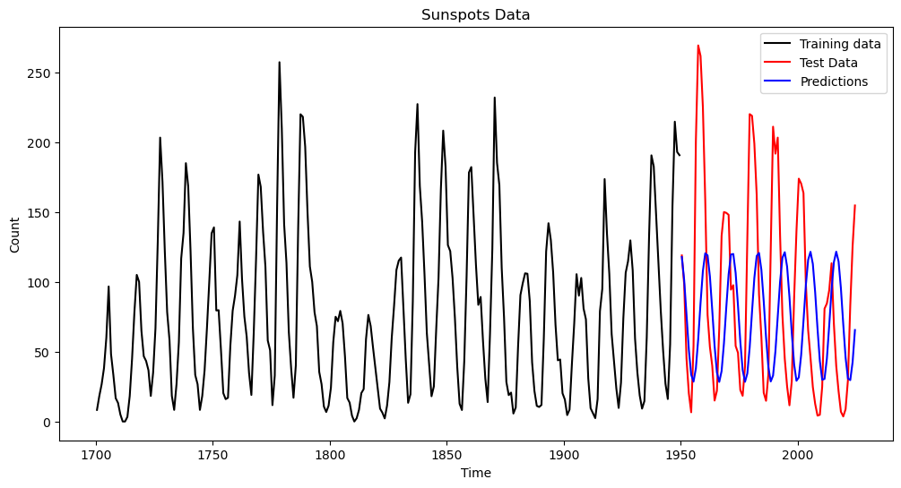
Model Two: The Yule Model
This model is motivated by the following observation (discussed with proof in Lecture 16) that
is equivalent to (below )
This suggests that a different sinusoid plus noise model is obtained by adding noise in the above equation leading to:
The parameters and can be fit by least squares by minimizing
Note that the time index goes from 3 to above (because we do not have access to and/or when ). This least squares estimator can be computed by creating a new response variable and regressing it on (and the constant term).
p = 2
yreg = y[p:]
x1 = y[1:-1]
x2 = y[:-2]
Xmat = np.column_stack([np.ones(len(yreg)), x1])

print(Xmat.shape)
(248, 2)
y_adjusted = yreg + x2
yulemod = sm.OLS(y_adjusted, Xmat).fit()

print(yulemod.summary())
print(yulemod.params)
OLS Regression Results
==============================================================================
Dep. Variable: y R-squared: 0.926
Model: OLS Adj. R-squared: 0.926
Method: Least Squares F-statistic: 3090.
Date: Thu, 20 Mar 2025 Prob (F-statistic): 2.78e-141
Time: 20:49:50 Log-Likelihood: -1168.0
No. Observations: 248 AIC: 2340.
Df Residuals: 246 BIC: 2347.
Df Model: 1
Covariance Type: nonrobust
==============================================================================
coef std err t P>|t| [0.025 0.975]
------------------------------------------------------------------------------
const 27.3114 2.791 9.787 0.000 21.815 32.808
x1 1.6348 0.029 55.592 0.000 1.577 1.693
==============================================================================
Omnibus: 10.450 Durbin-Watson: 2.408
Prob(Omnibus): 0.005 Jarque-Bera (JB): 20.195
Skew: 0.133 Prob(JB): 4.12e-05
Kurtosis: 4.372 Cond. No. 155.
==============================================================================
Notes:
[1] Standard Errors assume that the covariance matrix of the errors is correctly specified.
[27.31136502 1.634765 ]
Because , we can obtain an estimate of from the least squares estimate of obtained above.
alpha1_hat = yulemod.params[1]
yulefhat = np.arccos(alpha1_hat/2) / (2 * np.pi)

print(1/yulefhat)
10.234141128185033
It is interesting that the period corresponding to this estimate of is less than 11 by a nontrivial amount.
We now obtain predictions for the test times from the Yule model.
# Generate k-step ahead forecasts:
k = len(tme_test)
yhat = np.concatenate([y, np.full(k, -9999)]) # extend data by k placeholder values

for i in range(1, k+1):
    ans = yulemod.params[0] - yhat[n+i-3]
    ans += yulemod.params[1] * yhat[n+i-2]
    yhat[n+i-1] = ans

predvalues_yulemod = yhat[n:]
print(predvalues_yulemod)
[146.06104972 75.38685636 4.49010921 -40.73521796 -43.77125261
-3.50912861 65.34601702 137.64587487 186.98400606 195.34039803
159.66300392 92.98245693 19.65282692 -33.5433384 -47.17693735
-16.26850237 47.89312417 121.87387032 178.65337795 197.49378336
171.513911 110.20251965 35.9526756 -24.11697905 -48.06690374
-27.14974761 30.99481172 105.13034589 168.17996275 197.11573524
181.36930636 126.69182313 53.05341637 -12.65059012 -46.42279325
-35.92840227 14.99966389 87.76069276 155.77980967 194.21405216
189.02588952 142.11022034 70.60228927 0.6192958 -42.27852115
-42.42337723 0.23763408 70.12321812 141.70871333 188.84859105
194.32571784 156.13965529 88.2372901 15.41894292 -35.71957693
-46.50069192 -12.98676148 52.58175387 126.25693714 181.13003247
197.15946465 168.49072395 105.59463801 31.44305903 -26.88126073
-48.07623808 -24.4007254 35.49815135 109.74322567 171.21759752
197.46867444 178.90864425 122.31627964 48.36109315 -15.94589238]
plt.figure(figsize = (12, 6))
plt.xlabel('Time')
plt.ylabel('Count')
plt.plot(tme, sunspots.iloc[:,1], color = "None")
plt.plot(tme_train, y, color = 'black', label = 'Training data')
plt.plot(tme_test, sunspots_test.iloc[:,1], color = 'red', label = 'Test Data')
#plt.plot(tme_test, pred_test, color = 'blue', label = 'Predictions (Model One)')
plt.plot(tme_test, predvalues_yulemod, color = 'green', label = 'Predictions (Model Two)')
plt.legend()
plt.title('Sunspots Data')
plt.show() 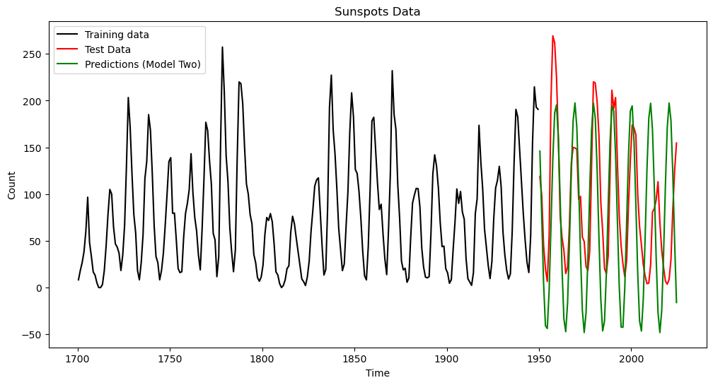
pred_error_rms_yulemod = np.sqrt(np.mean((predvalues_yulemod - sunspots_test.iloc[:,1]) ** 2))
print(pred_error_rms_sinusoid, pred_error_rms_yulemod)
#basically the same prediction errors (slightly smaller for the Yule model); expect different results for different training-test splits.
79.83531765284938 79.52702577862316
Model Three: AR(2)
The AR(2) model is a natural extension of the Yule model:
The only difference between the Yule model and AR(2) is that in the Yule model while it is treated as an adjustable parameter which can provide better fits to the data in AR(2).
The AR(2) model is fit in the following way.
p = 2
yreg = y[p:] # these are the response values in the autoregression
Xmat = np.ones((n-p, 1)) # this will be the design matrix (X) in the autoregression

for j in range(1, p+1):
    col = y[p-j : n-j].reshape(-1, 1)
    Xmat = np.column_stack([Xmat, col])
armod = sm.OLS(yreg, Xmat).fit()
print(armod.params)
print(armod.summary())
sighat = np.sqrt(np.mean(armod.resid ** 2))
print(sighat)[23.08524521 1.37838349 -0.68406411]
OLS Regression Results
==============================================================================
Dep. Variable: y R-squared: 0.822
Model: OLS Adj. R-squared: 0.821
Method: Least Squares F-statistic: 567.0
Date: Thu, 20 Mar 2025 Prob (F-statistic): 1.19e-92
Time: 20:45:50 Log-Likelihood: -1147.2
No. Observations: 248 AIC: 2300.
Df Residuals: 245 BIC: 2311.
Df Model: 2
Covariance Type: nonrobust
==============================================================================
coef std err t P>|t| [0.025 0.975]
------------------------------------------------------------------------------
const 23.0852 2.647 8.722 0.000 17.872 28.299
x1 1.3784 0.047 29.399 0.000 1.286 1.471
x2 -0.6841 0.047 -14.506 0.000 -0.777 -0.591
==============================================================================
Omnibus: 25.182 Durbin-Watson: 2.117
Prob(Omnibus): 0.000 Jarque-Bera (JB): 37.915
Skew: 0.631 Prob(JB): 5.85e-09
Kurtosis: 4.441 Cond. No. 220.
==============================================================================
Notes:
[1] Standard Errors assume that the covariance matrix of the errors is correctly specified.
24.697886587075086
Note that the estimated value of (which is the value of which gives the best fit to the data in the least squares sense) is -0.6841 which is quite a bit smaller than the value of -1 which is hard-coded in the Yule model.
Let us obtain predictions for the future values using the fitted AR(2) model.
# Generate k-step ahead forecasts:
k = len(tme_test)
yhat = np.concatenate([y, np.full(k, -9999)]) # extend data by k placeholder values

for i in range(1, k+1):
    ans = armod.params[0]
    for j in range(1, p+1):
        ans += armod.params[j] * yhat[n+i-j-1]

    yhat[n+i-1] = ans

predvalues_ar = yhat[n:]
plt.figure(figsize = (12, 6))
plt.xlabel('Time')
plt.ylabel('Count')
plt.plot(tme, sunspots.iloc[:,1], color = "None")
plt.plot(tme_train, y, color = 'black', label = 'Training data')
plt.plot(tme_test, sunspots_test.iloc[:,1], color = 'red', label = 'Test Data')
plt.plot(tme_test, pred_test, color = 'blue', label = 'Predictions (Model One)')
plt.plot(tme_test, predvalues_yulemod, color = 'green', label = 'Predictions (Model Two)')
plt.plot(tme_test, predvalues_ar, color = 'yellow', label = 'Predictions (Model Three)')
plt.legend()
plt.title('Sunspots Data')
plt.show() 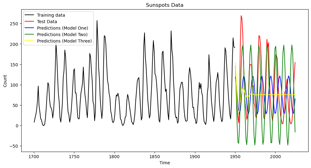
The predictions look quite different. For AR(2), the predictions die out to a constant value.
pred_error_rms_ar = np.sqrt(np.mean((predvalues_ar - sunspots_test.iloc[:,1]) ** 2))
print(pred_error_rms_sinusoid, pred_error_rms_yulemod, pred_error_rms_ar)
79.83531765284938 79.52702577862316 70.32365837557232
It is interesting that even though the predictions of the AR model die out to a constant value, in terms of prediction accuracy, it performs better than the previous two sinusoidal models. One reason for this is that the cycles of the sunspots data are irregular (and their periodicity changes from cycle to cycle). If we use a single sinusoid for prediction (as in Models One and Two), there is a danger that the predictions go out of phase with the actual data. The AR model, by predicting a constant, becomes more accurate than a sinusoidal model that goes out of phase. Note though that this prediction comparison will change if we change the training and test datasets.
Model Four: AR() for a higher 
We can see how the predictions change if we use for a higher . The AR(p) for should give better fits to the data. Unless there is overfitting, this should lead to better predictions as well.
p = 12
yreg = y[p:] # these are the response values in the autoregression
Xmat = np.ones((n-p, 1)) # this will be the design matrix (X) in the autoregression

for j in range(1, p+1):
    col = y[p-j: n-j].reshape(-1, 1)
    Xmat = np.column_stack([Xmat, col])
armod = sm.OLS(yreg, Xmat).fit()
print(armod.params)
print(armod.summary())
sighat = np.sqrt(np.mean(armod.resid ** 2))
print(sighat)[13.12906966 1.21947938 -0.50695376 -0.10670251 0.16956741 -0.15634832
0.05883931 -0.05974739 0.10456934 0.09940318 -0.06642164 0.14368696
-0.06191045]
OLS Regression Results
==============================================================================
Dep. Variable: y R-squared: 0.850
Model: OLS Adj. R-squared: 0.842
Method: Least Squares F-statistic: 106.0
Date: Thu, 20 Mar 2025 Prob (F-statistic): 2.00e-85
Time: 20:45:50 Log-Likelihood: -1082.3
No. Observations: 238 AIC: 2191.
Df Residuals: 225 BIC: 2236.
Df Model: 12
Covariance Type: nonrobust
==============================================================================
coef std err t P>|t| [0.025 0.975]
------------------------------------------------------------------------------
const 13.1291 4.789 2.742 0.007 3.693 22.565
x1 1.2195 0.067 18.239 0.000 1.088 1.351
x2 -0.5070 0.106 -4.795 0.000 -0.715 -0.299
x3 -0.1067 0.112 -0.957 0.340 -0.327 0.113
x4 0.1696 0.112 1.517 0.131 -0.051 0.390
x5 -0.1563 0.113 -1.389 0.166 -0.378 0.065
x6 0.0588 0.112 0.525 0.600 -0.162 0.280
x7 -0.0597 0.111 -0.540 0.590 -0.278 0.158
x8 0.1046 0.110 0.951 0.343 -0.112 0.321
x9 0.0994 0.109 0.908 0.365 -0.116 0.315
x10 -0.0664 0.109 -0.608 0.544 -0.282 0.149
x11 0.1437 0.105 1.372 0.171 -0.063 0.350
x12 -0.0619 0.067 -0.922 0.358 -0.194 0.070
==============================================================================
Omnibus: 30.370 Durbin-Watson: 1.990
Prob(Omnibus): 0.000 Jarque-Bera (JB): 51.328
Skew: 0.713 Prob(JB): 7.15e-12
Kurtosis: 4.773 Cond. No. 859.
==============================================================================
Notes:
[1] Standard Errors assume that the covariance matrix of the errors is correctly specified.
22.837160267072164
# Generate k-step ahead forecasts:
k = len(tme_test)
yhat = np.concatenate([y, np.full(k, -9999)]) # extend data by k placeholder values

for i in range(1, k+1):
    ans = armod.params[0]
    for j in range(1, p+1):
        ans += armod.params[j] * yhat[n+i-j-1]

    yhat[n+i-1] = ans

predvalues_ar_high = yhat[n:]
pred_error_rms_ar_high = np.sqrt(np.mean((predvalues_ar_high - sunspots_test.iloc[:,1]) ** 2))
print(pred_error_rms_sinusoid, pred_error_rms_yulemod,
pred_error_rms_ar, pred_error_rms_ar_high)79.83531765284938 79.52702577862316 70.32365837557232 50.162969939451386
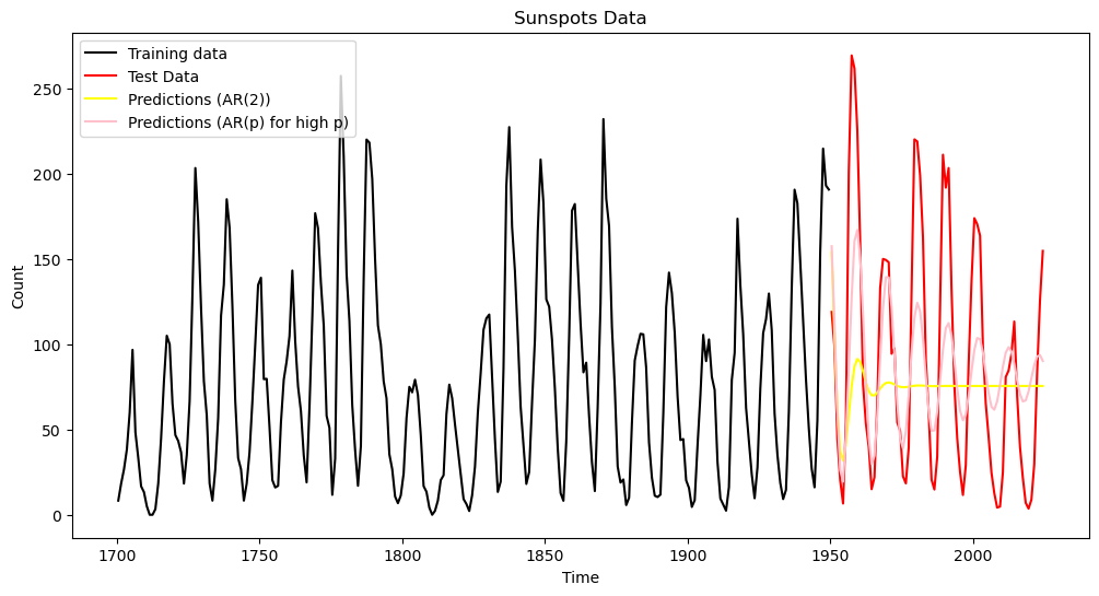
With , the prediction accuracy is much better compared to (as well as models 1 and 2).
plt.figure(figsize = (12, 6))
plt.xlabel('Time')
plt.ylabel('Count')
plt.plot(tme, sunspots.iloc[:,1], color = "None")
plt.plot(tme_train, y, color = 'black', label = 'Training data')
plt.plot(tme_test, sunspots_test.iloc[:,1], color = 'red', label = 'Test Data')
#plt.plot(tme_test, pred_test, color = 'blue', label = 'Predictions (Model One)')
#plt.plot(tme_test, predvalues_yulemod, color = 'green', label = 'Predictions (Model Two)')
plt.plot(tme_test, predvalues_ar, color = 'yellow', label = 'Predictions (AR(2))')
plt.plot(tme_test, predvalues_ar_high, color = 'pink', label = 'Predictions (AR(p) for high p)')
plt.legend()
plt.title('Sunspots Data')
plt.show()