import pandas as pd
uspop = pd.read_csv("POPTHM-Jan2025FRED.csv")
y = uspop['POPTHM']
n = len(y)
import numpy as np
x = np.arange(1, n + 1)
X = np.column_stack([np.ones(n), x])
print(y[:5])
print(X[:5])
0 175818
1 176044
2 176274
3 176503
4 176723
Name: POPTHM, dtype: int64
[[1. 1.]
[1. 2.]
[1. 3.]
[1. 4.]
[1. 5.]]
import statsmodels.api as sm
linmod = sm.OLS(y, X).fit()
print(linmod.summary())
OLS Regression Results
==============================================================================
Dep. Variable: POPTHM R-squared: 0.997
Model: OLS Adj. R-squared: 0.997
Method: Least Squares F-statistic: 2.422e+05
Date: Thu, 30 Jan 2025 Prob (F-statistic): 0.00
Time: 19:54:04 Log-Likelihood: -7394.9
No. Observations: 791 AIC: 1.479e+04
Df Residuals: 789 BIC: 1.480e+04
Df Model: 1
Covariance Type: nonrobust
==============================================================================
coef std err t P>|t| [0.025 0.975]
------------------------------------------------------------------------------
const 1.746e+05 198.060 881.427 0.000 1.74e+05 1.75e+05
x1 213.2353 0.433 492.142 0.000 212.385 214.086
==============================================================================
Omnibus: 409.683 Durbin-Watson: 0.000
Prob(Omnibus): 0.000 Jarque-Bera (JB): 73.601
Skew: -0.479 Prob(JB): 1.04e-16
Kurtosis: 1.853 Cond. No. 915.
==============================================================================
Notes:
[1] Standard Errors assume that the covariance matrix of the errors is correctly specified.
import matplotlib.pyplot as plt
plt.plot(y)
plt.plot(linmod.fittedvalues)
plt.xlabel('Time (monthly)')
plt.ylabel('Thousands')
plt.title('Monthly US population')
plt.show()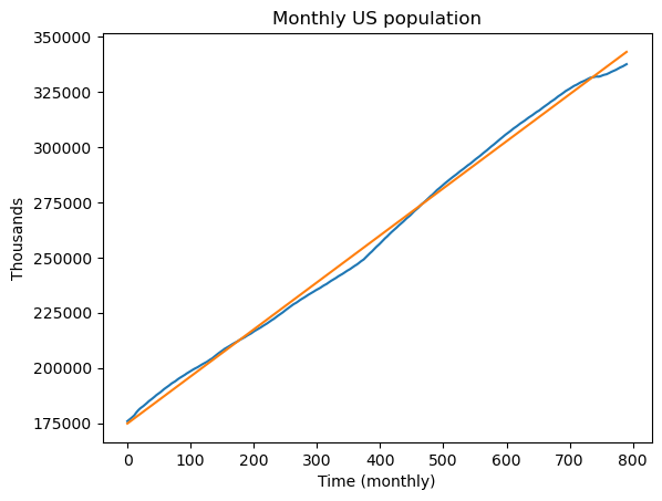
#the coefficient estimates are:
print(linmod.params)
print(linmod.cov_params())
const 174575.148609
x1 213.235255
dtype: float64
const x1
const 39227.640424 -74.341706
x1 -74.341706 0.187732
sighat = np.sqrt(np.sum(linmod.resid ** 2)/(n - 2))
XT = X.T
XTX = np.dot(XT, X)
XTX_inverse = np.linalg.inv(XTX)
covmat = (sighat ** 2) * XTX_inverse
print(covmat)
[[ 3.92276404e+04 -7.43417064e+01]
[-7.43417064e+01 1.87731582e-01]]
#Drawing posterior samples:
help(np.random.Generator.multivariate_normal)
N = 1000 #number of desired posterior samples
rng = np.random.default_rng()
samples_normalposterior = rng.multivariate_normal(mean = linmod.params, cov = linmod.cov_params(), size = N)
print(samples_normalposterior)[[174270.47890247 213.30305805]
[174921.21639834 212.59386417]
[174800.67256417 212.86154695]
...
[174435.25565323 213.53607588]
[174718.07536863 212.93705101]
[174937.11713602 212.68556081]]
import matplotlib.pyplot as plt
plt.scatter(samples_normalposterior[:,0], samples_normalposterior[:,1], marker = '.')
plt.xlabel('Intercept')
plt.ylabel('Slope')
plt.title('Posterior Samples (drawn from normal approximation)')
plt.show()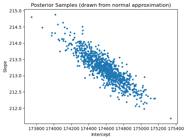
N = 2000 #number of desired posterior samples
rng = np.random.default_rng()
samples_normalposterior = rng.multivariate_normal(mean = linmod.params, cov = linmod.cov_params(), size = N)
demean_samples_normalposterior = samples_normalposterior - np.array(linmod.params)
chirvs = rng.chisquare(df = n-2, size = N)
samples_tposterior = np.zeros((N, 2))
for r in range(N):
    samples_tposterior[r] = (np.array(linmod.params)) + (demean_samples_normalposterior[r]/(np.sqrt(chirvs[r]/(n-2))))
plt.scatter(samples_normalposterior[:,0], samples_normalposterior[:,1], marker = '.', label = 'Normal posterior')
plt.scatter(samples_tposterior[:,0], samples_tposterior[:,1], color = 'red', marker = '.', label = 't-posterior')
plt.xlabel('Intercept')
plt.ylabel('Slope')
plt.title('Posterior Samples (drawn from normal approximation)')
plt.legend()
plt.show()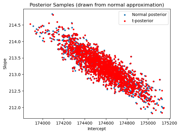
plt.plot(y)
for r in range(N):
fvalsnew = np.dot(X, samples_tposterior[r])
plt.plot(fvalsnew, color = 'red')
plt.plot(y, color = 'blue')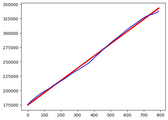
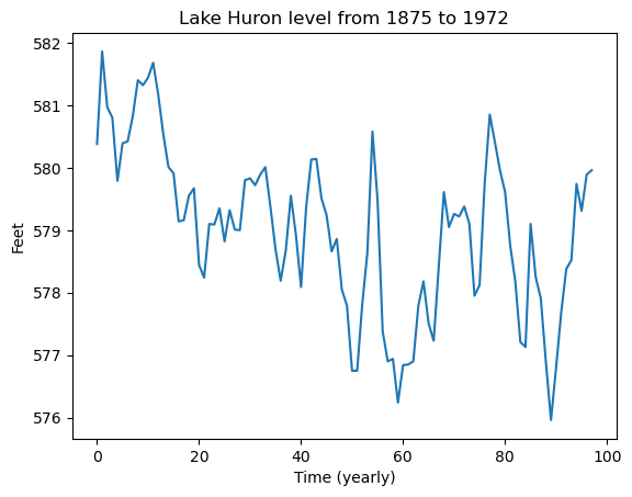
#Lake Huron dataset which gives annual measurements of the level (in feet) of Lake Huron from 1875 to 1972
huron = pd.read_csv("LakeHuron.csv")
print(huron)
plt.plot(huron['x'])
plt.xlabel('Time (yearly)')
plt.ylabel('Feet')
plt.title('Lake Huron level from 1875 to 1972')
plt.show() Unnamed: 0 x
0 1 580.38
1 2 581.86
2 3 580.97
3 4 580.80
4 5 579.79
.. ... ...
93 94 578.52
94 95 579.74
95 96 579.31
96 97 579.89
97 98 579.96
[98 rows x 2 columns]
y = huron['x']
n = len(y)
x = np.arange(1, n+1)
X = np.column_stack([np.ones(n), x])
print(X)[[ 1. 1.]
[ 1. 2.]
[ 1. 3.]
[ 1. 4.]
[ 1. 5.]
[ 1. 6.]
[ 1. 7.]
[ 1. 8.]
[ 1. 9.]
[ 1. 10.]
[ 1. 11.]
[ 1. 12.]
[ 1. 13.]
[ 1. 14.]
[ 1. 15.]
[ 1. 16.]
[ 1. 17.]
[ 1. 18.]
[ 1. 19.]
[ 1. 20.]
[ 1. 21.]
[ 1. 22.]
[ 1. 23.]
[ 1. 24.]
[ 1. 25.]
[ 1. 26.]
[ 1. 27.]
[ 1. 28.]
[ 1. 29.]
[ 1. 30.]
[ 1. 31.]
[ 1. 32.]
[ 1. 33.]
[ 1. 34.]
[ 1. 35.]
[ 1. 36.]
[ 1. 37.]
[ 1. 38.]
[ 1. 39.]
[ 1. 40.]
[ 1. 41.]
[ 1. 42.]
[ 1. 43.]
[ 1. 44.]
[ 1. 45.]
[ 1. 46.]
[ 1. 47.]
[ 1. 48.]
[ 1. 49.]
[ 1. 50.]
[ 1. 51.]
[ 1. 52.]
[ 1. 53.]
[ 1. 54.]
[ 1. 55.]
[ 1. 56.]
[ 1. 57.]
[ 1. 58.]
[ 1. 59.]
[ 1. 60.]
[ 1. 61.]
[ 1. 62.]
[ 1. 63.]
[ 1. 64.]
[ 1. 65.]
[ 1. 66.]
[ 1. 67.]
[ 1. 68.]
[ 1. 69.]
[ 1. 70.]
[ 1. 71.]
[ 1. 72.]
[ 1. 73.]
[ 1. 74.]
[ 1. 75.]
[ 1. 76.]
[ 1. 77.]
[ 1. 78.]
[ 1. 79.]
[ 1. 80.]
[ 1. 81.]
[ 1. 82.]
[ 1. 83.]
[ 1. 84.]
[ 1. 85.]
[ 1. 86.]
[ 1. 87.]
[ 1. 88.]
[ 1. 89.]
[ 1. 90.]
[ 1. 91.]
[ 1. 92.]
[ 1. 93.]
[ 1. 94.]
[ 1. 95.]
[ 1. 96.]
[ 1. 97.]
[ 1. 98.]]
linmod = sm.OLS(y, X).fit()
print(linmod.summary()) OLS Regression Results
==============================================================================
Dep. Variable: x R-squared: 0.272
Model: OLS Adj. R-squared: 0.265
Method: Least Squares F-statistic: 35.95
Date: Thu, 30 Jan 2025 Prob (F-statistic): 3.55e-08
Time: 16:52:56 Log-Likelihood: -150.05
No. Observations: 98 AIC: 304.1
Df Residuals: 96 BIC: 309.3
Df Model: 1
Covariance Type: nonrobust
==============================================================================
coef std err t P>|t| [0.025 0.975]
------------------------------------------------------------------------------
const 580.2020 0.230 2521.398 0.000 579.745 580.659
x1 -0.0242 0.004 -5.996 0.000 -0.032 -0.016
==============================================================================
Omnibus: 1.626 Durbin-Watson: 0.439
Prob(Omnibus): 0.444 Jarque-Bera (JB): 1.274
Skew: -0.039 Prob(JB): 0.529
Kurtosis: 2.447 Cond. No. 115.
==============================================================================
Notes:
[1] Standard Errors assume that the covariance matrix of the errors is correctly specified.
N = 2000 #number of desired posterior samples
rng = np.random.default_rng()
samples_normalposterior = rng.multivariate_normal(mean = linmod.params, cov = linmod.cov_params(), size = N)
demean_samples_normalposterior = samples_normalposterior - np.array(linmod.params)
chirvs = rng.chisquare(df = n-2, size = N)
samples_tposterior = np.zeros((N, 2))
for r in range(N):
samples_tposterior[r] = (np.array(linmod.params)) + (demean_samples_normalposterior[r]/(np.sqrt(chirvs[r]/(n-2))))
plt.plot(y)
for r in range(N):
fvalsnew = np.dot(X, samples_tposterior[r])
plt.plot(fvalsnew, color = 'red')
plt.plot(y, color = 'blue')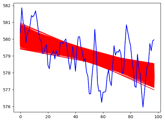
plt.scatter(samples_normalposterior[:,0], samples_normalposterior[:,1], marker = '.', label = 'Normal posterior')
plt.scatter(samples_tposterior[:,0], samples_tposterior[:,1], color = 'red', marker = '.', label = 't-posterior')
plt.xlabel('Intercept')
plt.ylabel('Slope')
plt.title('Posterior Samples (drawn from normal approximation)')
plt.legend()
plt.show()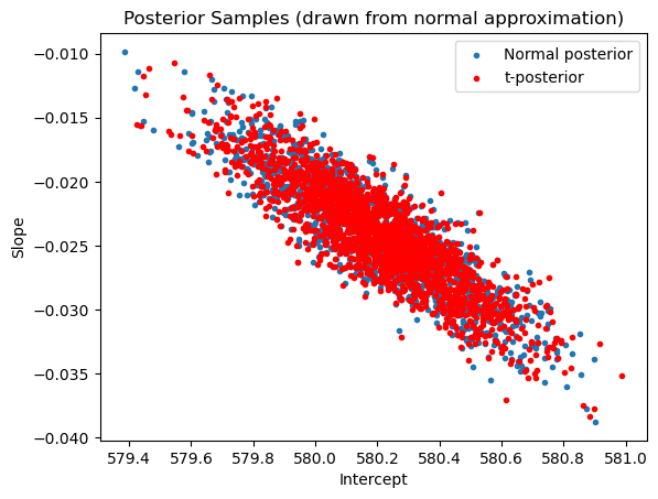
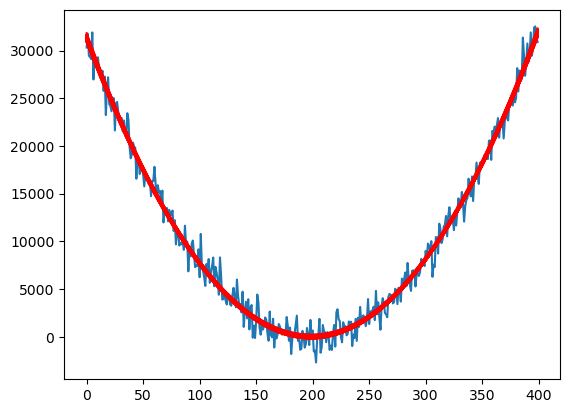
#A simulated dataset
n = 400
x = np.arange(1, n+1)
sig = 1000
y = 5 + 0.8 * ((x - (n/2)) ** 2) + rng.normal(loc = 0, scale = sig, size = n)
plt.plot(y)
plt.xlabel("Time")
plt.ylabel("Data")
plt.title("A simulated dataset")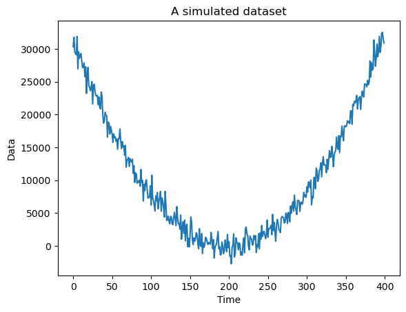
X = np.column_stack([np.ones(n), x])
linmod = sm.OLS(y, X).fit()
plt.plot(y)
plt.plot(linmod.fittedvalues, color = "red")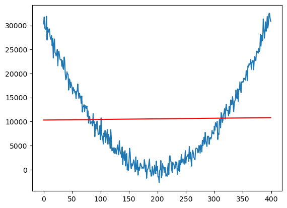
N = 200 #number of desired posterior samples
rng = np.random.default_rng()
samples_normalposterior = rng.multivariate_normal(mean = linmod.params, cov = linmod.cov_params(), size = N)
demean_samples_normalposterior = samples_normalposterior - np.array(linmod.params)
chirvs = rng.chisquare(df = n-2, size = N)
samples_tposterior = np.zeros((N, 2))
for r in range(N):
samples_tposterior[r] = (np.array(linmod.params)) + (demean_samples_normalposterior[r]/(np.sqrt(chirvs[r]/(n-2))))
plt.plot(y)
for r in range(N):
    fvalsnew = np.dot(X, samples_tposterior[r])
    plt.plot(fvalsnew,  color = 'red')
plt.plot(y, color = 'blue')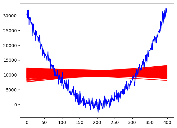
X  = np.column_stack([np.ones(n), x, x ** 2])
quadmod = sm.OLS(y, X).fit()
N = 200 #number of desired posterior samples
rng = np.random.default_rng()
samples_normalposterior = rng.multivariate_normal(mean = quadmod.params, cov = quadmod.cov_params(), size = N)
demean_samples_normalposterior = samples_normalposterior - np.array(quadmod.params)
chirvs = rng.chisquare(df = n-3, size = N)
samples_tposterior = np.zeros((N, 3))
for r in range(N):
    samples_tposterior[r] = (np.array(quadmod.params)) + (demean_samples_normalposterior[r]/(np.sqrt(chirvs[r]/(n-3))))
plt.plot(y)
for r in range(N):
    fvalsnew = np.dot(X, samples_tposterior[r])
    plt.plot(fvalsnew,  color = 'red')
#plt.plot(y, color = 'blue')