import numpy as np
import pandas as pd
import matplotlib.pyplot as plt
import statsmodels.api as sm
We fit AR models by OLS of on where is the vector consisting of and consists of rows for . This gives rise to estimates which are also known as Conditional MLEs or Conditional Least Squares Estimates (conditional here refers to conditioning on ).
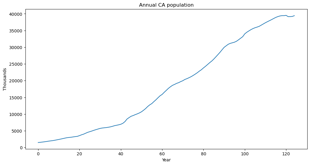
Dataset One: California Population
#California Population Dataset from FRED
capop = pd.read_csv('CAPOP_20March2025.csv')
print(capop.head())
y = capop['CAPOP'].to_numpy()
n = len(y)
print(n)
plt.figure(figsize = (12, 6))
plt.plot(y)
plt.xlabel('Year')
plt.ylabel('Thousands')
plt.title('Annual CA population')
plt.show()
observation_date CAPOP
0 1900-01-01 1490.0
1 1901-01-01 1550.0
2 1902-01-01 1623.0
3 1903-01-01 1702.0
4 1904-01-01 1792.0
125
We can AR(p) models to this data using the following code.
p = 1
n = len(y)
yreg = y[p:] #these are the response values in the autoregression
Xmat = np.ones((n-p, 1)) #this will be the design matrix (X) in the autoregression
for j in range(1, p+1):
    col = y[p-j : n-j].reshape(-1, 1)
    Xmat = np.column_stack([Xmat, col])

armod = sm.OLS(yreg, Xmat).fit()
print(armod.params)
print(armod.summary())
sighat = np.sqrt(np.mean(armod.resid ** 2))
print(sighat)
[236.66072866 1.0038257 ]
OLS Regression Results
==============================================================================
Dep. Variable: y R-squared: 1.000
Model: OLS Adj. R-squared: 1.000
Method: Least Squares F-statistic: 5.574e+05
Date: Sat, 22 Mar 2025 Prob (F-statistic): 4.02e-225
Time: 14:56:55 Log-Likelihood: -828.87
No. Observations: 124 AIC: 1662.
Df Residuals: 122 BIC: 1667.
Df Model: 1
Covariance Type: nonrobust
==============================================================================
coef std err t P>|t| [0.025 0.975]
------------------------------------------------------------------------------
const 236.6607 30.009 7.886 0.000 177.255 296.066
x1 1.0038 0.001 746.589 0.000 1.001 1.006
==============================================================================
Omnibus: 5.372 Durbin-Watson: 0.342
Prob(Omnibus): 0.068 Jarque-Bera (JB): 8.010
Skew: 0.028 Prob(JB): 0.0182
Kurtosis: 4.244 Cond. No. 3.82e+04
==============================================================================
Notes:
[1] Standard Errors assume that the covariance matrix of the errors is correctly specified.
[2] The condition number is large, 3.82e+04. This might indicate that there are
strong multicollinearity or other numerical problems.
193.54270158976897
Instead of creating and and then using OLS, we can fit AR(p) model directly using the AutoReg function in statsmodels.
from statsmodels.tsa.ar_model import AutoReg
armod_sm = AutoReg(y, lags = p, trend = 'c').fit()
print(armod_sm.summary())
AutoReg Model Results
==============================================================================
Dep. Variable: y No. Observations: 125
Model: AutoReg(1) Log Likelihood -828.870
Method: Conditional MLE S.D. of innovations 193.543
Date: Sat, 22 Mar 2025 AIC 1663.740
Time: 14:56:56 BIC 1672.201
Sample: 1 HQIC 1667.177
125
==============================================================================
coef std err z P>|z| [0.025 0.975]
------------------------------------------------------------------------------
const 236.6607 29.766 7.951 0.000 178.321 295.001
y.L1 1.0038 0.001 752.683 0.000 1.001 1.006
Roots
=============================================================================
Real Imaginary Modulus Frequency
-----------------------------------------------------------------------------
AR.1 0.9962 +0.0000j 0.9962 0.0000
-----------------------------------------------------------------------------
Note that “Method: Conditional MLE” in the above output. The estimates of and are the same in both outputs above.
The fitted model leads to predictions for future observations which can be calculated as follows.
#Generate k-step ahead forecasts:
k = 100 #increase k to see exponential behavior in AR(1) predictions
yhat = np.concatenate([y, np.full(k, -9999)]) #extend data by k placeholder values
phi_vals = armod.params
for i in range(1, k+1):
    ans = phi_vals[0]
    for j in range(1, p+1):
        ans += phi_vals[j] * yhat[n+i-j-1]
    yhat[n+i-1] = ans
predvalues = yhat[n:]

#Plotting the series with forecasts:
plt.figure(figsize=(12, 6))
time_all = np.arange(1, n + k + 1)
plt.plot(time_all, yhat, color='C0')
plt.plot(range(1, n + 1), y, label='Original Data', color='C1')
plt.plot(range(n + 1, n + k + 1), predvalues, label='Forecasts', color='blue')
plt.axvline(x=n, color='black', linestyle='--', label='Forecast Start')
#plt.axhline(y=np.mean(y), color='gray', linestyle=':', label='Mean of Original Data')
plt.xlabel('Time')
plt.ylabel('Data')
plt.title('Time Series + AR(p) Forecasts')
plt.legend()
plt.show()
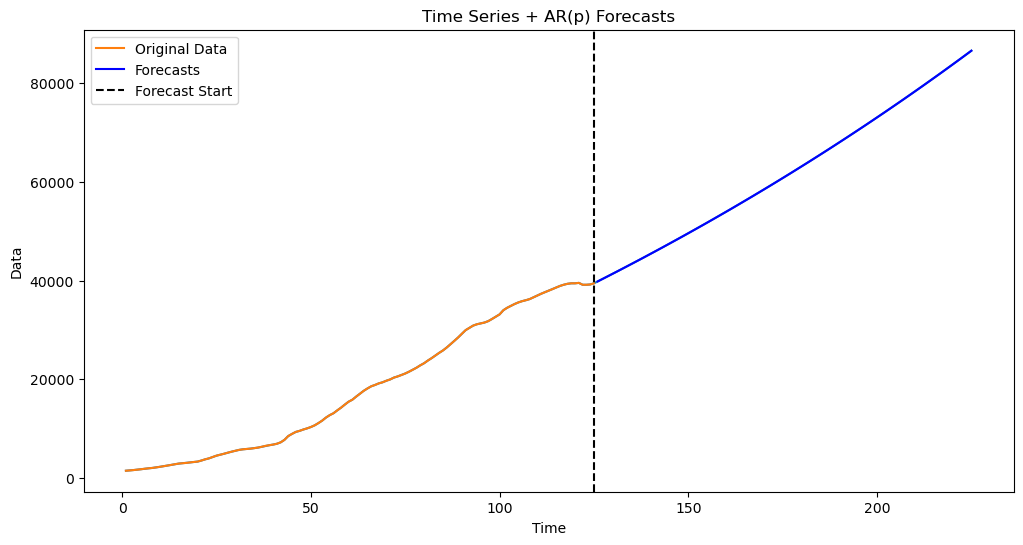
In this AR(1) model, the fitted estimate is slightly more than 1. So the predictions are exponential. If you increase , this exponential behaviour will be become visible (when is small, the predictions look linear).
The same predictions are obtained from the AutoReg object using the predict function.
predvalues_sm = armod_sm.predict(start = n, end = n+k-1)
yhat = np.concatenate([y, predvalues_sm])
Check below that both predictions lead to the same values.
plt.figure(figsize=(12, 6))
time_all = np.arange(1, n + k + 1)
plt.plot(time_all, yhat, color='C0', label="Extended Series with Forecasts")
plt.plot(range(1, n + 1), y, label='Original Data', color='C1')
plt.plot(range(n + 1, n + k + 1), predvalues_sm, label='Forecasts (Statsmodels AutoReg)', color='blue')
plt.plot(range(n + 1, n + k + 1), predvalues, label='Forecasts (OLS)', color='green')
plt.axvline(x=n, color='black', linestyle='--', label='Forecast Start')
plt.xlabel('Time')
plt.ylabel('Data')
plt.title('Time Series + AR(p) Forecasts')
plt.legend()
plt.show()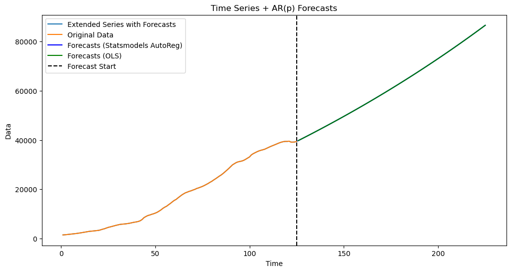
When changes, the predictions change appreciably. Run the code below for various values of to see how the predictions change.
p = 1 #large p e.g., p = 25 leads to predictions that decrease into the future.
armod_sm = AutoReg(y, lags = p, trend = 'c').fit()
print(armod_sm.summary())
predvalues_sm = armod_sm.predict(start = n, end = n+k-1)
yhat = np.concatenate([y, predvalues_sm])
plt.figure(figsize=(12, 6))
time_all = np.arange(1, n + k + 1)
plt.plot(time_all, yhat, color='C0', label="Extended Series with Forecasts")
plt.plot(range(1, n + 1), y, label='Original Data', color='C1')
plt.plot(range(n + 1, n + k + 1), predvalues_sm, label='Forecasts (Statsmodels AutoReg)', color='blue')
plt.axvline(x=n, color='black', linestyle='--', label='Forecast Start')
plt.xlabel('Time')
plt.ylabel('Data')
plt.title('Time Series + AR(p) Forecasts')
plt.legend()
plt.show()
AutoReg Model Results
==============================================================================
Dep. Variable: y No. Observations: 125
Model: AutoReg(25) Log Likelihood -601.595
Method: Conditional MLE S.D. of innovations 99.188
Date: Sat, 22 Mar 2025 AIC 1257.190
Time: 15:01:01 BIC 1327.530
Sample: 25 HQIC 1285.658
125
==============================================================================
coef std err z P>|z| [0.025 0.975]
------------------------------------------------------------------------------
const 48.5749 31.228 1.555 0.120 -12.632 109.782
y.L1 1.7693 0.100 17.607 0.000 1.572 1.966
y.L2 -0.5359 0.204 -2.632 0.008 -0.935 -0.137
y.L3 -0.3854 0.207 -1.860 0.063 -0.792 0.021
y.L4 0.0123 0.207 0.060 0.952 -0.393 0.417
y.L5 0.0966 0.218 0.442 0.658 -0.331 0.525
y.L6 0.0967 0.221 0.437 0.662 -0.337 0.530
y.L7 -0.0334 0.221 -0.151 0.880 -0.466 0.399
y.L8 0.1527 0.220 0.695 0.487 -0.278 0.583
y.L9 -0.3617 0.220 -1.643 0.100 -0.793 0.070
y.L10 0.3859 0.223 1.734 0.083 -0.050 0.822
y.L11 -0.2041 0.226 -0.903 0.366 -0.647 0.239
y.L12 -0.2265 0.226 -1.000 0.317 -0.670 0.217
y.L13 0.3839 0.224 1.715 0.086 -0.055 0.823
y.L14 -0.0488 0.226 -0.216 0.829 -0.492 0.394
y.L15 -0.0288 0.225 -0.128 0.898 -0.470 0.412
y.L16 -0.2512 0.222 -1.134 0.257 -0.686 0.183
y.L17 0.0877 0.221 0.396 0.692 -0.346 0.521
y.L18 0.1523 0.222 0.687 0.492 -0.282 0.587
y.L19 0.1106 0.222 0.498 0.619 -0.325 0.546
y.L20 -0.0222 0.221 -0.100 0.920 -0.456 0.412
y.L21 -0.7083 0.221 -3.201 0.001 -1.142 -0.275
y.L22 0.9305 0.233 3.997 0.000 0.474 1.387
y.L23 -0.4332 0.251 -1.726 0.084 -0.925 0.059
y.L24 0.1580 0.243 0.650 0.516 -0.318 0.634
y.L25 -0.0995 0.119 -0.838 0.402 -0.332 0.133
Roots
==============================================================================
Real Imaginary Modulus Frequency
------------------------------------------------------------------------------
AR.1 -1.0075 -0.0000j 1.0075 -0.5000
AR.2 -0.9809 -0.2737j 1.0183 -0.4567
AR.3 -0.9809 +0.2737j 1.0183 0.4567
AR.4 -0.8328 -0.5853j 1.0179 -0.4025
AR.5 -0.8328 +0.5853j 1.0179 0.4025
AR.6 -0.6709 -0.7787j 1.0278 -0.3632
AR.7 -0.6709 +0.7787j 1.0278 0.3632
AR.8 -0.3740 -0.9839j 1.0526 -0.3078
AR.9 -0.3740 +0.9839j 1.0526 0.3078
AR.10 -0.1016 -1.0310j 1.0360 -0.2656
AR.11 -0.1016 +1.0310j 1.0360 0.2656
AR.12 0.2724 -0.9824j 1.0195 -0.2069
AR.13 0.2724 +0.9824j 1.0195 0.2069
AR.14 0.6190 -0.8776j 1.0739 -0.1522
AR.15 0.6190 +0.8776j 1.0739 0.1522
AR.16 0.7994 -0.6917j 1.0571 -0.1135
AR.17 0.7994 +0.6917j 1.0571 0.1135
AR.18 0.9170 -0.4919j 1.0406 -0.0784
AR.19 0.9170 +0.4919j 1.0406 0.0784
AR.20 1.0284 -0.2495j 1.0582 -0.0379
AR.21 1.0284 +0.2495j 1.0582 0.0379
AR.22 0.9984 -0.0240j 0.9987 -0.0038
AR.23 0.9984 +0.0240j 0.9987 0.0038
AR.24 -0.3772 -2.1016j 2.1352 -0.2783
AR.25 -0.3772 +2.1016j 2.1352 0.2783
------------------------------------------------------------------------------
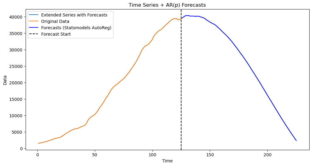
When is large (e.g., ), check that the predictions decrease in time. Given that the dataset here is small (), the AR(25) model overfits and its predictions are not reliable.
Dataset Two: simulated dataset
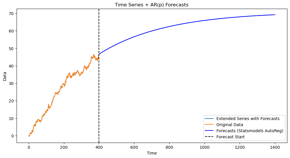
AR(1) predictions behave quite differently in the three regimes , and . To see this, consider the simulated dataset below.
seed = 43
rng = np.random.default_rng(seed)
n = 400
sig = 0.5
ysim = np.zeros(n)
for i in range(2, n):
    err = rng.normal(loc = 0, scale = sig, size = 1)
    phi_0 = 0.1
    phi_1 = 1
    ysim[i] = phi_0 + phi_1 * ysim[i-1] + err[0]
plt.figure(figsize = (12, 6))
plt.plot(ysim)
plt.show()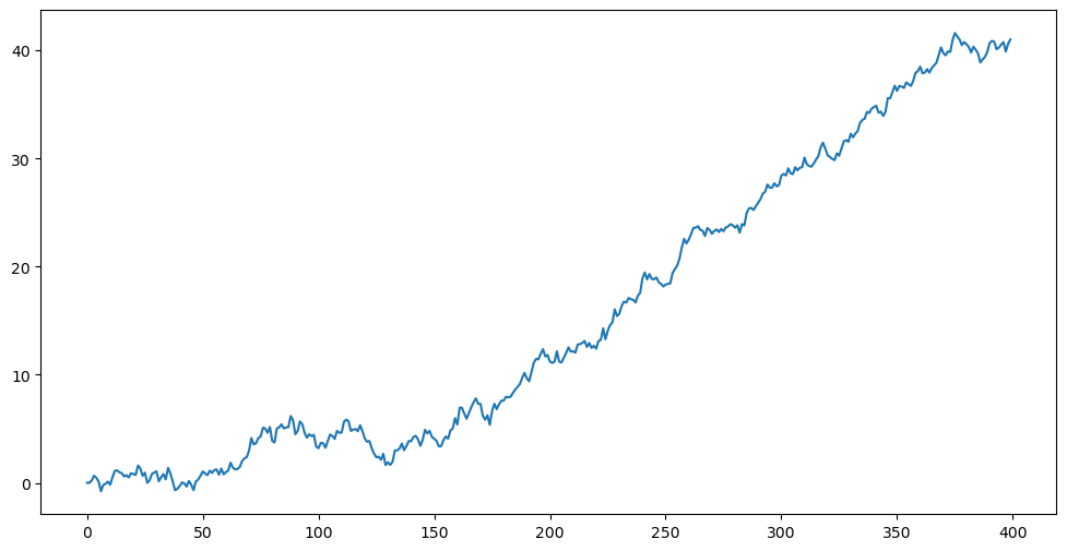
p = 1
armod_sm = AutoReg(ysim, lags = p, trend = 'c').fit()
print(armod_sm.summary())
k = 1000
predvalues_sm = armod_sm.predict(start = n, end = n+k-1)
yhat = np.concatenate([ysim, predvalues_sm])
plt.figure(figsize=(12, 6))
time_all = np.arange(1, n + k + 1)
plt.plot(time_all, yhat, color='C0', label="Extended Series with Forecasts")
plt.plot(range(1, n + 1), ysim, label='Original Data', color='C1')
plt.plot(range(n + 1, n + k + 1), predvalues_sm, label='Forecasts (Statsmodels AutoReg)', color='blue')
plt.axvline(x=n, color='black', linestyle='--', label='Forecast Start')
plt.xlabel('Time')
plt.ylabel('Data')
plt.title('Time Series + AR(p) Forecasts')
plt.legend()
plt.show()
AutoReg Model Results
==============================================================================
Dep. Variable: y No. Observations: 400
Model: AutoReg(1) Log Likelihood -283.472
Method: Conditional MLE S.D. of innovations 0.492
Date: Sat, 22 Mar 2025 AIC 572.945
Time: 15:05:19 BIC 584.911
Sample: 1 HQIC 577.684
400
==============================================================================
coef std err z P>|z| [0.025 0.975]
------------------------------------------------------------------------------
const 0.0705 0.037 1.891 0.059 -0.003 0.144
y.L1 1.0021 0.002 555.249 0.000 0.999 1.006
Roots
=============================================================================
Real Imaginary Modulus Frequency
-----------------------------------------------------------------------------
AR.1 0.9979 +0.0000j 0.9979 0.0000
-----------------------------------------------------------------------------
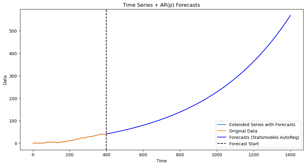
The estimated is more than 1 and the predictions are exponential. If we forcibly set the parameter to be 1, the predictions will be linear. This is done below.
k = 1000
yhat = np.concatenate([ysim, np.full(k, -9999)]) #extend data by k placeholder values
phi_vals = np.array([armod_sm.params[0], 1]) #\phi_1 parameter is set to 1
for i in range(1, k+1):
    ans = phi_vals[0]
    for j in range(1, p+1):
        ans += phi_vals[j] * yhat[n+i-j-1]
    yhat[n+i-1] = ans
predvalues = yhat[n:]

#Plotting the series with forecasts:
plt.figure(figsize=(12, 6))
time_all = np.arange(1, n + k + 1)
plt.plot(time_all, yhat, color='C0')
plt.plot(range(1, n + 1), ysim, label='Original Data', color='C1')
plt.plot(range(n + 1, n + k + 1), predvalues, label='Forecasts', color='blue')
plt.axvline(x=n, color='black', linestyle='--', label='Forecast Start')
#plt.axhline(y=np.mean(y), color='gray', linestyle=':', label='Mean of Original Data')
plt.xlabel('Time')
plt.ylabel('Data')
plt.title('Time Series + AR(p) Forecasts')
plt.legend()
plt.show()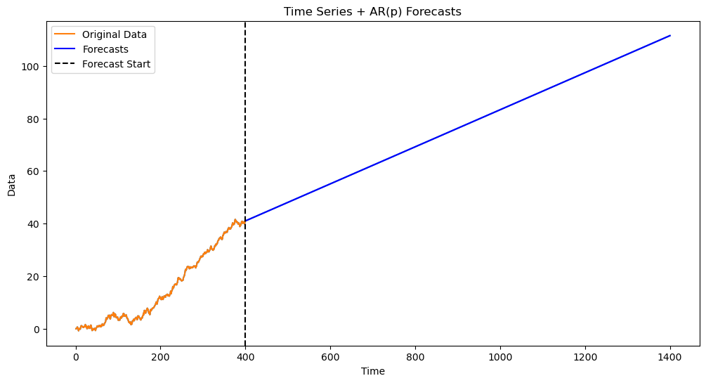
Now for the following simulated dataset, the estimated is slightly smaller than 1. This leads to predictions that decay to a constant.
seed = 123
rng = np.random.default_rng(seed)
n = 400
sig = 0.5
ysim = np.zeros(n)
for i in range(2, n):
    err = rng.normal(loc = 0, scale = sig, size = 1)
    phi_0 = 0.1
    phi_1 = 1
    ysim[i] = phi_0 + phi_1 * ysim[i-1] + err[0]
plt.figure(figsize = (12, 6))
plt.plot(ysim)
plt.show()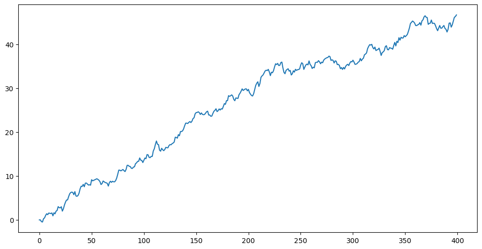
p = 1
armod_sm = AutoReg(ysim, lags = p, trend = 'c').fit()
print(armod_sm.summary())
k = 1000
predvalues_sm = armod_sm.predict(start = n, end = n+k-1)
yhat = np.concatenate([ysim, predvalues_sm])
plt.figure(figsize=(12, 6))
time_all = np.arange(1, n + k + 1)
plt.plot(time_all, yhat, color='C0', label="Extended Series with Forecasts")
plt.plot(range(1, n + 1), ysim, label='Original Data', color='C1')
plt.plot(range(n + 1, n + k + 1), predvalues_sm, label='Forecasts (Statsmodels AutoReg)', color='blue')
plt.axvline(x=n, color='black', linestyle='--', label='Forecast Start')
plt.xlabel('Time')
plt.ylabel('Data')
plt.title('Time Series + AR(p) Forecasts')
plt.legend()
plt.show()
AutoReg Model Results
==============================================================================
Dep. Variable: y No. Observations: 400
Model: AutoReg(1) Log Likelihood -289.700
Method: Conditional MLE S.D. of innovations 0.500
Date: Sat, 22 Mar 2025 AIC 585.400
Time: 15:06:45 BIC 597.367
Sample: 1 HQIC 590.140
400
==============================================================================
coef std err z P>|z| [0.025 0.975]
------------------------------------------------------------------------------
const 0.1857 0.055 3.391 0.001 0.078 0.293
y.L1 0.9974 0.002 538.039 0.000 0.994 1.001
Roots
=============================================================================
Real Imaginary Modulus Frequency
-----------------------------------------------------------------------------
AR.1 1.0026 +0.0000j 1.0026 0.0000
-----------------------------------------------------------------------------
Again, if we force to equal 1, the predictions will be linear.
k = 1000
yhat = np.concatenate([ysim, np.full(k, -9999)]) #extend data by k placeholder values
phi_vals = np.array([armod_sm.params[0], 1]) #\phi_1 parameter is set to 1
for i in range(1, k+1):
    ans = phi_vals[0]
    for j in range(1, p+1):
        ans += phi_vals[j] * yhat[n+i-j-1]
    yhat[n+i-1] = ans
predvalues = yhat[n:]

#Plotting the series with forecasts:
plt.figure(figsize=(12, 6))
time_all = np.arange(1, n + k + 1)
plt.plot(time_all, yhat, color='C0')
plt.plot(range(1, n + 1), ysim, label='Original Data', color='C1')
plt.plot(range(n + 1, n + k + 1), predvalues, label='Forecasts', color='blue')
plt.axvline(x=n, color='black', linestyle='--', label='Forecast Start')
#plt.axhline(y=np.mean(y), color='gray', linestyle=':', label='Mean of Original Data')
plt.xlabel('Time')
plt.ylabel('Data')
plt.title('Time Series + AR(p) Forecasts')
plt.legend()
plt.show()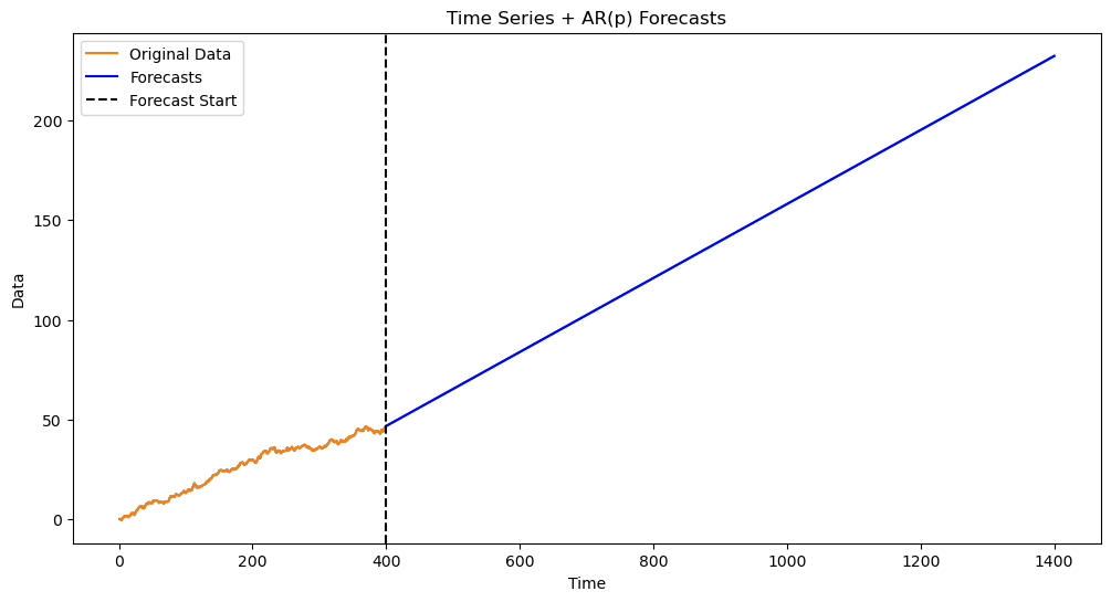
Dataset Three: Sunspots
Predictions for AR(2) have a more richer structure than those for AR(1). In some examples (such as the sunspots dataset), AR(2) will result in predictions that oscillate (a behaviour which will never be seen in predictions for AR(1)).
sunspots = pd.read_csv('SN_y_tot_V2.0.csv', header = None, sep = ';')
y = sunspots.iloc[:,1].values
n = len(y)
plt.figure(figsize = (12, 6))
plt.plot(y)
plt.show()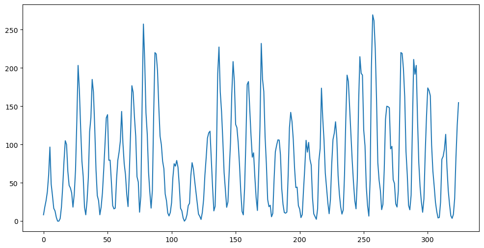
Let us fit AR(2) model to this data.
armod_sm = AutoReg(y, lags = 2, trend = 'c').fit()
print(armod_sm.summary())
AutoReg Model Results
==============================================================================
Dep. Variable: y No. Observations: 325
Model: AutoReg(2) Log Likelihood -1505.524
Method: Conditional MLE S.D. of innovations 25.588
Date: Sat, 22 Mar 2025 AIC 3019.048
Time: 15:10:14 BIC 3034.159
Sample: 2 HQIC 3025.080
325
==============================================================================
coef std err z P>|z| [0.025 0.975]
------------------------------------------------------------------------------
const 24.4561 2.372 10.308 0.000 19.806 29.106
y.L1 1.3880 0.040 34.685 0.000 1.310 1.466
y.L2 -0.6965 0.040 -17.423 0.000 -0.775 -0.618
Roots
=============================================================================
Real Imaginary Modulus Frequency
-----------------------------------------------------------------------------
AR.1 0.9965 -0.6655j 1.1983 -0.0937
AR.2 0.9965 +0.6655j 1.1983 0.0937
-----------------------------------------------------------------------------
Predictions generated by the fitted AR(2) are plotted below.
p = 2
armod_sm = AutoReg(y, lags = p, trend = 'c').fit()
print(armod_sm.summary())
k = 100
predvalues_sm = armod_sm.predict(start = n, end = n+k-1)
yhat = np.concatenate([y, predvalues_sm])
plt.figure(figsize=(12, 6))
time_all = np.arange(1, n + k + 1)
plt.plot(time_all, yhat, color='C0', label="Extended Series with Forecasts")
plt.plot(range(1, n + 1), y, label='Original Data', color='C1')
plt.plot(range(n + 1, n + k + 1), predvalues_sm, label='Forecasts (Statsmodels AutoReg)', color='blue')
plt.axvline(x=n, color='black', linestyle='--', label='Forecast Start')
plt.xlabel('Time')
plt.ylabel('Data')
plt.title('Time Series + AR(p) Forecasts')
plt.legend()
plt.show()
AutoReg Model Results
==============================================================================
Dep. Variable: y No. Observations: 325
Model: AutoReg(2) Log Likelihood -1505.524
Method: Conditional MLE S.D. of innovations 25.588
Date: Sat, 22 Mar 2025 AIC 3019.048
Time: 15:10:15 BIC 3034.159
Sample: 2 HQIC 3025.080
325
==============================================================================
coef std err z P>|z| [0.025 0.975]
------------------------------------------------------------------------------
const 24.4561 2.372 10.308 0.000 19.806 29.106
y.L1 1.3880 0.040 34.685 0.000 1.310 1.466
y.L2 -0.6965 0.040 -17.423 0.000 -0.775 -0.618
Roots
=============================================================================
Real Imaginary Modulus Frequency
-----------------------------------------------------------------------------
AR.1 0.9965 -0.6655j 1.1983 -0.0937
AR.2 0.9965 +0.6655j 1.1983 0.0937
-----------------------------------------------------------------------------
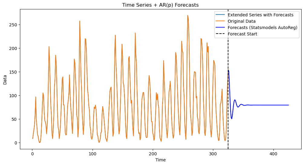
The oscillating nature of the predictions are clearly visible above. We shall see some formulae (next lecture) for AR(2) predictions that explain this oscillating predictions.