import numpy as np
import pandas as pd
import matplotlib.pyplot as plt
US Population Dataset
The following dataset is downloaded from the Federal Reserve Economic Database FRED (https://
uspop = pd.read_csv("POPTHM-Jan2025FRED.csv")
print(uspop.head(10))
print(uspop.tail(10))
print(uspop.shape)
observation_date POPTHM
0 1959-01-01 175818
1 1959-02-01 176044
2 1959-03-01 176274
3 1959-04-01 176503
4 1959-05-01 176723
5 1959-06-01 176954
6 1959-07-01 177208
7 1959-08-01 177479
8 1959-09-01 177755
9 1959-10-01 178026
observation_date POPTHM
781 2024-02-01 336306
782 2024-03-01 336423
783 2024-04-01 336550
784 2024-05-01 336687
785 2024-06-01 336839
786 2024-07-01 337005
787 2024-08-01 337185
788 2024-09-01 337362
789 2024-10-01 337521
790 2024-11-01 337669
(791, 2)
plt.plot(uspop['POPTHM'])
plt.xlabel("Time (in months)")
plt.ylabel("Population (in thousands)")
plt.title("US Population Data")
plt.show()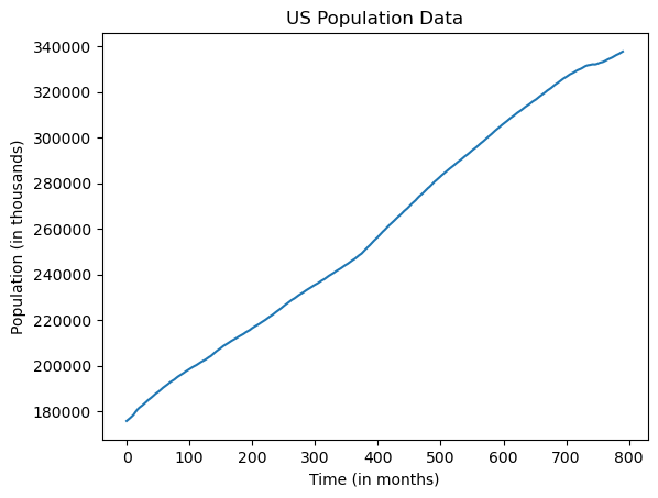
Problem 1
Fit a simple linear regression model to the data. Interpret the estimated intercept and slope.
import statsmodels.api as sm

t = np.arange(1, len(uspop['POPTHM']) + 1)
X = sm.add_constant(t)

lin_model = sm.OLS(uspop['POPTHM'], X).fit()
print(lin_model.summary())
OLS Regression Results
==============================================================================
Dep. Variable: POPTHM R-squared: 0.997
Model: OLS Adj. R-squared: 0.997
Method: Least Squares F-statistic: 2.422e+05
Date: Thu, 23 Jan 2025 Prob (F-statistic): 0.00
Time: 23:54:49 Log-Likelihood: -7394.9
No. Observations: 791 AIC: 1.479e+04
Df Residuals: 789 BIC: 1.480e+04
Df Model: 1
Covariance Type: nonrobust
==============================================================================
coef std err t P>|t| [0.025 0.975]
------------------------------------------------------------------------------
const 1.746e+05 198.060 881.427 0.000 1.74e+05 1.75e+05
x1 213.2353 0.433 492.142 0.000 212.385 214.086
==============================================================================
Omnibus: 409.683 Durbin-Watson: 0.000
Prob(Omnibus): 0.000 Jarque-Bera (JB): 73.601
Skew: -0.479 Prob(JB): 1.04e-16
Kurtosis: 1.853 Cond. No. 915.
==============================================================================
Notes:
[1] Standard Errors assume that the covariance matrix of the errors is correctly specified.
# Plot the original dataset along with the fitted values
plt.figure(figsize = (10, 6))
plt.plot(t, uspop['POPTHM'], label = 'US population', color = 'blue')
plt.plot(t, lin_model.fittedvalues, label = 'Linear Fit', color = 'red')
plt.xlabel("Time (months)")
plt.ylabel("US Population (in thousands)")
plt.title("US Population")
plt.legend()
plt.show()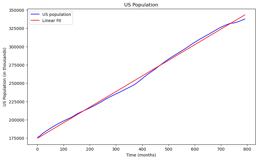
USA Accidents Dataset
This dataset was inbuilt in R. I have saved it as “USAccDeaths.csv”.
USAccDeaths = pd.read_csv("USAccDeaths.csv")
print(USAccDeaths.head(10))
print(USAccDeaths.tail(10))
print(USAccDeaths.shape)
Unnamed: 0 x
0 1 9007
1 2 8106
2 3 8928
3 4 9137
4 5 10017
5 6 10826
6 7 11317
7 8 10744
8 9 9713
9 10 9938
Unnamed: 0 x
62 63 7791
63 64 8192
64 65 9115
65 66 9434
66 67 10484
67 68 9827
68 69 9110
69 70 9070
70 71 8633
71 72 9240
(72, 2)
dt = USAccDeaths['x']
plt.plot(dt)
plt.xlabel("Time (months) from 1973 to 1978")
plt.ylabel("Number of accidental deaths")
plt.title("Number of accidental deaths in  USA")
plt.show() 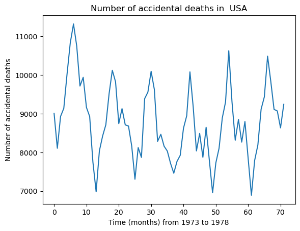
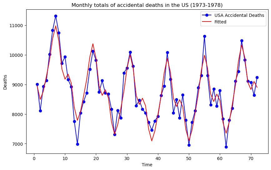
Problem 2
Fit a sinusoids + quadratic multiple regression model to the data.
t = np.arange(1, len(dt) + 1)

f1, f2, f3 = 1, 2, 3
d = 12

v1 = np.cos(2 * np.pi * f1 * t/d)
v2 = np.sin(2 * np.pi * f1 * t/d)
v3 = np.cos(2 * np.pi * f2 * t/d)
v4 = np.sin(2 * np.pi * f2 * t/d)
v5 = np.cos(2 * np.pi * f3 * t/d)
v6 = np.sin(2 * np.pi * f3 * t/d)

v7 = t
v8 = t ** 2

X = np.column_stack([v1, v2, v3, v4, v5, v6, v7, v8])
X = sm.add_constant(X)

lin_mod = sm.OLS(dt, X).fit()
print(lin_mod.summary())

plt.figure(figsize = (10, 6))
plt.plot(t, dt, label = "USA Accidental Deaths", marker = 'o', linestyle = '-', color = 'blue')
plt.plot(t, lin_mod.fittedvalues, label = 'Fitted', color = 'red', linestyle = '-')
plt.xlabel("Time")
plt.ylabel("Deaths")
plt.title("Monthly totals of accidental deaths in the US (1973-1978)")
plt.legend()
plt.show()
OLS Regression Results
==============================================================================
Dep. Variable: x R-squared: 0.881
Model: OLS Adj. R-squared: 0.866
Method: Least Squares F-statistic: 58.54
Date: Thu, 23 Jan 2025 Prob (F-statistic): 2.93e-26
Time: 23:54:49 Log-Likelihood: -519.15
No. Observations: 72 AIC: 1056.
Df Residuals: 63 BIC: 1077.
Df Model: 8
Covariance Type: nonrobust
==============================================================================
coef std err t P>|t| [0.025 0.975]
------------------------------------------------------------------------------
const 9957.8596 127.837 77.895 0.000 9702.397 1.02e+04
x1 -734.1366 58.404 -12.570 0.000 -850.847 -617.426
x2 -757.6844 58.832 -12.879 0.000 -875.250 -640.119
x3 417.1503 58.386 7.145 0.000 300.476 533.825
x4 75.5988 58.454 1.293 0.201 -41.213 192.410
x5 156.7378 58.385 2.685 0.009 40.065 273.411
x6 -198.0336 58.385 -3.392 0.001 -314.706 -81.361
x7 -72.0713 8.056 -8.946 0.000 -88.171 -55.972
x8 0.8285 0.107 7.752 0.000 0.615 1.042
==============================================================================
Omnibus: 1.222 Durbin-Watson: 2.216
Prob(Omnibus): 0.543 Jarque-Bera (JB): 1.034
Skew: -0.043 Prob(JB): 0.596
Kurtosis: 2.419 Cond. No. 7.33e+03
==============================================================================
Notes:
[1] Standard Errors assume that the covariance matrix of the errors is correctly specified.
[2] The condition number is large, 7.33e+03. This might indicate that there are
strong multicollinearity or other numerical problems.