import numpy as np
import pandas as pd
import matplotlib.pyplot as plt
import torch
import torch.nn as nn
import torch.optim as optim
from statsmodels.tsa.ar_model import AutoReg
import statsmodels.api as sm
The following dataset is simulated according to the model:
for some fixed . This equation is for . For , we take to be linear. We take to be a large value.
n = 1500
truelag = 85
rng = np.random.default_rng(seed=0)
#sig_noise = 0.05
sig_noise = 0.01

eps = rng.normal(loc=0, scale=sig_noise, size=n)
y_sim = np.full(shape=n, fill_value=-999.0)
y_sim[0:truelag] = np.linspace(-1, 1, truelag)
for i in range(truelag, n):
    y_sim[i] = 0.9 * np.sin(0.5 * np.pi * y_sim[i - truelag]) + eps[i]
#y_sim = y_sim + eps

plt.figure(figsize = (12, 6))
plt.plot(y_sim)
plt.show()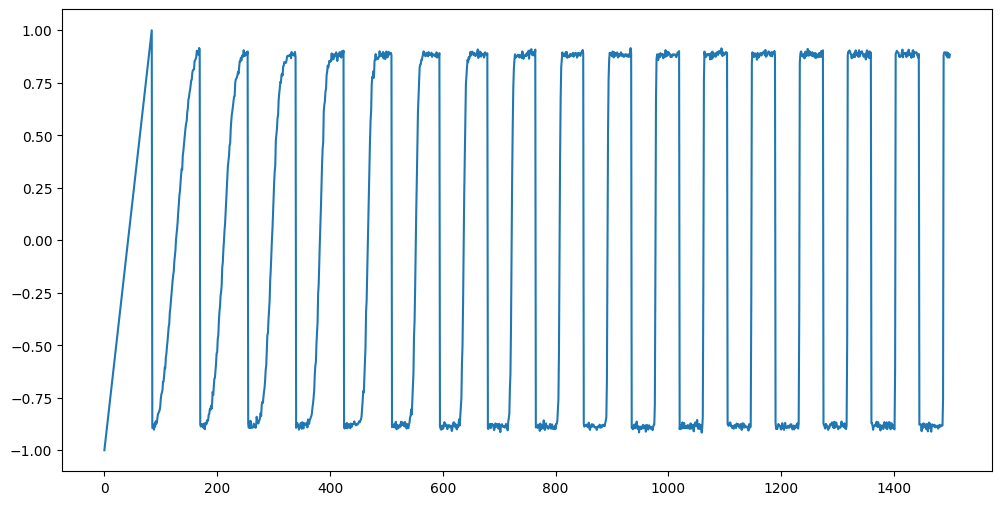
Let us obtain predictions for future values using the actual function from which the data were generated. These predictions (which we can refer to as Oracle Predictions) will form the benchmark which we can use to compare the predictions of various methods (AR, LSTM, RNN, GRU).
# Oracle Predictions
n_future = 1000
y_extended = np.concatenate([y_sim, np.empty(n_future, dtype=float)])
for t in range(n, n+n_future):
    y_extended[t] = 0.9 * np.sin(0.5 * np.pi * y_extended[t - truelag])
oracle_preds = y_extended[n:]

n = len(y_sim)
tme = range(1, n+1)
tme_future = range(n+1, n+n_future+1)

plt.figure(figsize = (12, 6))
plt.plot(tme, y_sim, label = 'Data')
plt.plot(tme_future, oracle_preds, label = 'Forecast (Oracle)', color = 'green')
plt.axvline(x=n, color='gray', linestyle='--')
plt.legend()
plt.show()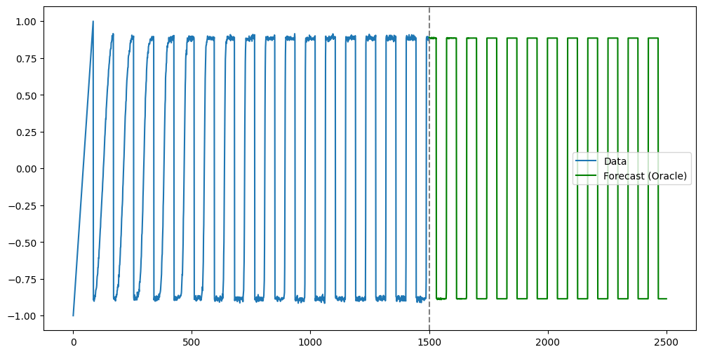
Let us now fit AR(p) to this data. Even if is taken to be the correct value, this model will not work well (because the actual function which generated the data is nonlinear).
# Let us fit AR(p)
p = truelag
#p = 50
ar = AutoReg(y_sim, lags=p).fit()

n = len(y_sim)
tme = range(1, n+1)
tme_future = range(n+1, n+n_future+1)
fcast = ar.get_prediction(start=n, end=n+n_future-1).predicted_mean

plt.figure(figsize = (12, 7))
plt.plot(tme, y_sim, label = 'Data')
plt.plot(tme_future, oracle_preds, label = 'Forecast (Oracle)', color = 'lightgreen')
plt.plot(tme_future, fcast, label = 'Forecast (AR(p))', color = 'black')
plt.axvline(x=n, color='gray', linestyle='--')
plt.legend()
plt.show()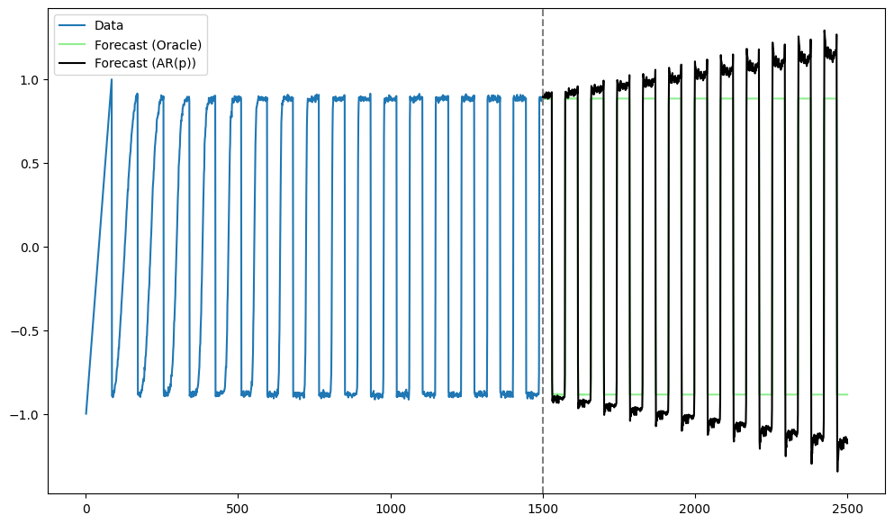
The AR predictions seem to be “expanding” compared to the Oracle predictions.
rmse_ar = np.sqrt(np.mean((fcast - oracle_preds)**2))
median_abs_error_ar = np.median(np.abs(fcast - oracle_preds))
print(rmse_ar)
print(median_abs_error_ar)
0.18216756914528526
0.1433347216860818
mu, sig = y_sim.mean(), y_sim.std()
y_std = (y_sim - mu) / sig

X = torch.tensor(y_std[:-1], dtype=torch.float32)
Y = torch.tensor(y_std[1: ], dtype=torch.float32)

X = X.unsqueeze(0).unsqueeze(-1)   # shape (1, seq_len, 1)
Y = Y.unsqueeze(0).unsqueeze(-1)   # shape (1, seq_len, 1)

seq_len = X.size(1)
print(seq_len)
1499
LSTM
The code below fits the LSTM, and uses it to obtain predictions.
class lstm_net(nn.Module):
    def __init__(self, nh):
        super().__init__()
        self.rnn = nn.LSTM(input_size=1, hidden_size=nh, batch_first=True)
        # input_size: the number of features in the input x
        # hidden_size: the number of features in the hidden state h(=r in our notation)
        # batch_first: If True, then the input and output tensors are provided
        #   as (batch, seq_len, feature) instead of (seq_len, batch, feature).
        #   In our case batch = 1, feature = 1
        self.fc  = nn.Linear(nh, 1)          # many-to-many

    def forward(self, x, hc=None):
        out, hc = self.rnn(x, hc)
        # out: (batch, seq_len, hidden_size)
        # hc = (h_n, c_n)
        #   the final hidden state h_n(=r_n) and c_n(=s_n in our notation)
        #   h_n: (1, hidden_size), c_n: (1, hidden_size)
        out     = self.fc(out)               # (batch, seq_len, 1)
        return out, hc

torch.manual_seed(0)
np.random.seed(0)

nh = 40
model = lstm_net(nh)
criterion = nn.MSELoss()
opt = torch.optim.Adam(model.parameters(), lr=1e-3)
n_epochs = 1000
for epoch in range(1, n_epochs + 1):
#model.train() # Set the model to training mode
opt.zero_grad()
pred, _ = model(X) # hidden state auto-reset every epoch
loss = criterion(pred, Y)
loss.backward()
opt.step()
if epoch % 100 == 0:
print(f"epoch {epoch:4d}/{n_epochs} | loss = {loss.item():.6f}")epoch 100/1000 | loss = 0.134661
epoch 200/1000 | loss = 0.068934
epoch 300/1000 | loss = 0.052071
epoch 400/1000 | loss = 0.054081
epoch 500/1000 | loss = 0.037171
epoch 600/1000 | loss = 0.029827
epoch 700/1000 | loss = 0.026267
epoch 800/1000 | loss = 0.023639
epoch 900/1000 | loss = 0.021077
epoch 1000/1000 | loss = 0.019640
#model.eval()

with torch.no_grad():
    _, hc = model(X)
    preds = np.zeros(n_future, dtype=np.float32)
    last_in = torch.tensor([[y_std[-1]]], dtype=torch.float32)  # (1, 1, 1) after view

    for t in range(n_future):
        out, hc = model(last_in.view(1, 1, 1), hc)              # reuse hidden state
        next_val = out.squeeze().item()
        preds[t] = next_val
        last_in = torch.tensor([[next_val]], dtype=torch.float32)
lstm_preds_orig = preds * sig + mu
tme_pred_axis = np.arange(n, n+n_future)
plt.figure(figsize=(12,6))
plt.plot(np.arange(n), y_sim, lw = 2, label = "Data")
plt.plot(tme_pred_axis, oracle_preds, color = 'lightgreen', label = 'Forecast (oracle)')
plt.plot(tme_pred_axis, lstm_preds_orig, lw = 2, color="r", label = "Forecast (LSTM)")
plt.plot(tme_pred_axis, fcast, lw = 2, color = "black", label = "Forecast (AR)")
plt.xlabel("Time"); plt.ylabel("Data")
plt.title("Data and Forecast")
plt.legend()
plt.tight_layout()
plt.show()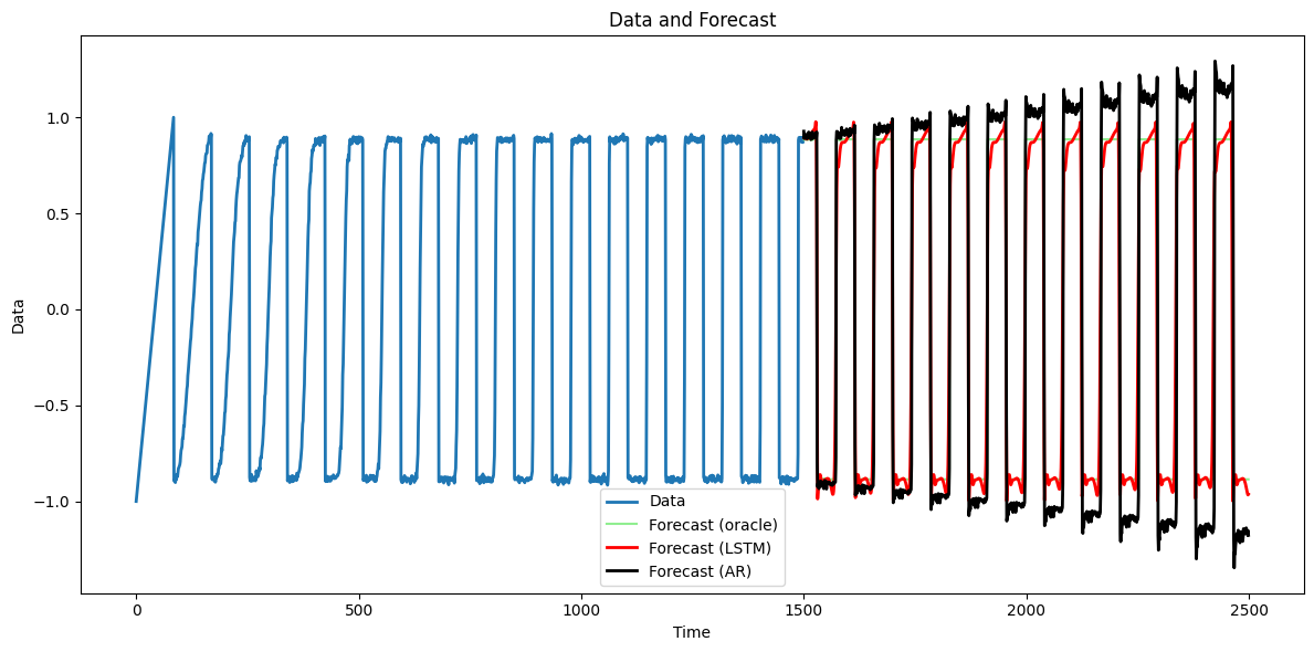
The LSTM predictions (with ) seem more reasonable compared to AR().
rmse_lstm = np.sqrt(np.mean((lstm_preds_orig - oracle_preds)**2))
median_abs_error_lstm = np.median(np.abs(lstm_preds_orig - oracle_preds))
print(rmse_ar, rmse_lstm)
print(median_abs_error_ar, median_abs_error_lstm)
0.18216756914528526 0.20501387820907402
0.1433347216860818 0.022898458729424975
Even though the predictions from LSTM are clearly better than those from AR as we can see from the plot above, AR produces smaller RMSE compared to LSTM. This is because the underlying function has many sharp tranisitions, and RMSE is sensitive to outlier error values. Even if LSTM generally performs well over the domain, a few large errors around the transition points can make RMSE larger. To address this issue, we can use more robust evaluation metrics. For example, we can think of using the median of absolute errors as we did above.
LSTM models can be quite unstable. To see this, go back to the simulation data and change sig_noise = 0.01 to sig_noise = 0 or sig_noise = 0.02, and see how the LSTM predictions change.
Presence of Trend
LSTM models do not work well where there is trend in the data. In such cases, remove the trend first (say by fitting a line and considering residuals) before fitting models.
n = 1500
truelag = 85
rng = np.random.default_rng(seed = 0)
#sig_noise = 0.05
sig_noise = 0.01

eps = rng.normal(loc=0, scale=sig_noise, size=n)
y_sim = np.full(shape=n, fill_value=-999.0)
y_sim[0:truelag] = np.linspace(-1, 1, truelag)
for i in range(truelag, n):
    y_sim[i] = 0.9 * np.sin(0.5 * np.pi * y_sim[i - truelag]) + eps[i]
#y_sim = y_sim + eps
y_sim = 0.001 * np.arange(1, n + 1) + y_sim

plt.figure(figsize = (12, 6))
plt.plot(y_sim)
plt.show()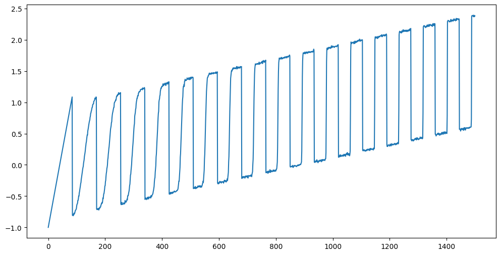
This data clearly has a linear trend. AR model will work well (as long as is correctly chosen).
# Let us fit AR(p)
p = truelag
ar = AutoReg(y_sim, lags=p).fit()

n = len(y_sim)
tme = range(1, n+1)
tme_future = range(n+1, n+n_future+1)
fcast = ar.get_prediction(start=n, end=n+n_future-1).predicted_mean

plt.figure(figsize = (12, 7))
plt.plot(tme, y_sim, label = 'Data')
plt.plot(tme_future, fcast, label = 'Forecast (AR(p))', color = 'black')
plt.axvline(x=n, color='gray', linestyle='--')
plt.legend()
plt.show()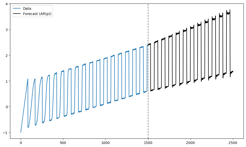
Now let us use LSTM for prediction.
mu, sig = y_sim.mean(), y_sim.std()
y_std = (y_sim - mu) / sig

X = torch.tensor(y_std[:-1], dtype=torch.float32)
Y = torch.tensor(y_std[1: ], dtype=torch.float32)

X = X.unsqueeze(0).unsqueeze(-1)   # shape (1, seq_len, 1)
Y = Y.unsqueeze(0).unsqueeze(-1)   # shape (1, seq_len, 1)

seq_len = X.size(1)
print(seq_len)
1499
class lstm_net(nn.Module):
    def __init__(self, nh):
        super().__init__()
        self.rnn = nn.LSTM(input_size=1, hidden_size=nh, batch_first=True)
        self.fc  = nn.Linear(nh, 1)      # many-to-many

    def forward(self, x, hc=None):
        out, hc = self.rnn(x, hc)        # out: (batch, seq_len, hidden_size)
        out     = self.fc(out)           # (batch, seq_len, 1)
        return out, hc

torch.manual_seed(0)
np.random.seed(0)

nh = 40
model = lstm_net(nh)
criterion = nn.MSELoss()
opt = torch.optim.Adam(model.parameters(), lr=1e-3)

n_epochs = 1000
for epoch in range(1, n_epochs + 1):
    #model.train()
    opt.zero_grad()

    pred, _ = model(X)           # hidden state auto-reset every epoch
    loss = criterion(pred, Y)
    loss.backward()

    opt.step()

    if epoch % 100 == 0:
        print(f"epoch {epoch:4d}/{n_epochs}  |  loss = {loss.item():.6f}")

#model.eval()
with torch.no_grad():
    _, hc = model(X)
    preds = np.zeros(n_future, dtype=np.float32)
    last_in = torch.tensor([[y_std[-1]]], dtype=torch.float32)  # (1, 1, 1) after view

    for t in range(n_future):
        out, hc = model(last_in.view(1, 1, 1), hc)              # reuse hidden state
        next_val = out.squeeze().item()
        preds[t] = next_val
        last_in = torch.tensor([[next_val]], dtype=torch.float32)

lstm_preds_orig = preds * sig + mu
tme_pred_axis = np.arange(n, n + n_future)

plt.figure(figsize=(12,6))
plt.plot(np.arange(n), y_sim, lw=2, label="Data")
plt.plot(tme_pred_axis, lstm_preds_orig, lw=2, color="r", label="Forecast (LSTM)")
plt.plot(tme_pred_axis, fcast, lw=2, color="black", label="Forecast (AR)")
plt.xlabel("Time"); plt.ylabel("Data")
plt.title("Data and Forecast")
plt.legend()
plt.tight_layout()
plt.show()
epoch 100/1000 | loss = 0.116244
epoch 200/1000 | loss = 0.076563
epoch 300/1000 | loss = 0.059973
epoch 400/1000 | loss = 0.054006
epoch 500/1000 | loss = 0.052959
epoch 600/1000 | loss = 0.050079
epoch 700/1000 | loss = 0.037976
epoch 800/1000 | loss = 0.038874
epoch 900/1000 | loss = 0.030605
epoch 1000/1000 | loss = 0.025062
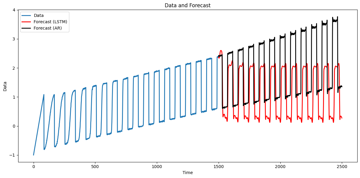
Clearly the predictions flatten out as the prediction horizon increases. This shows that detrending is recommended while working with LSTM models.
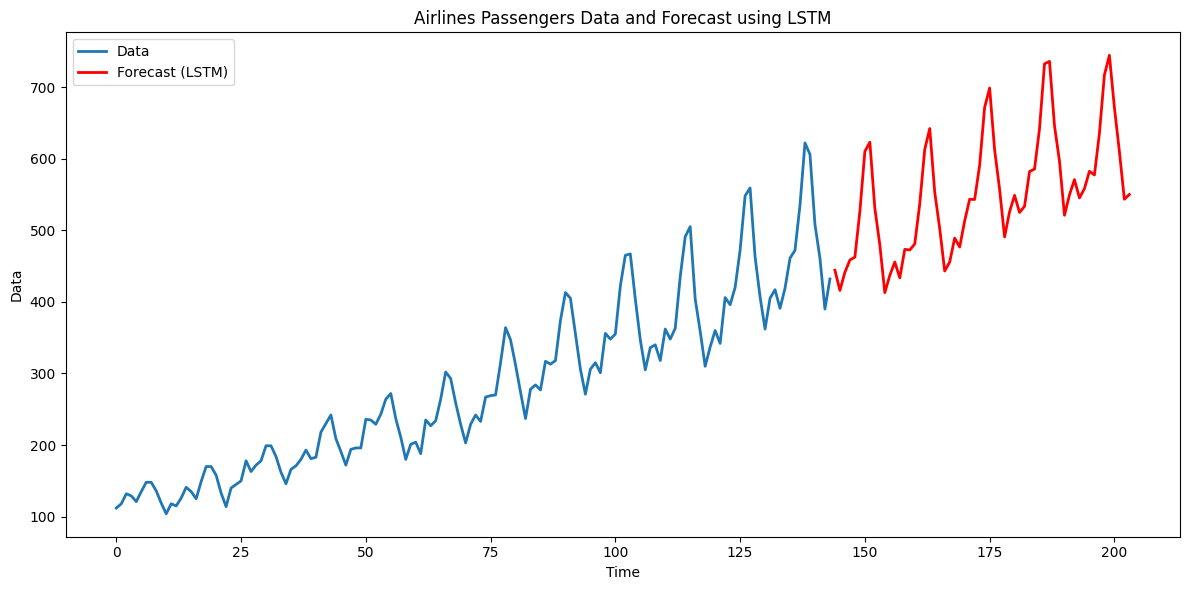
Airline Passengers Dataset
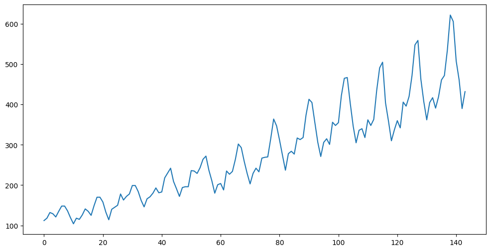
The airline passengers dataset is a popular dataset for evaluating prediction accuracy of various models. It contains monthly data on the number of international airline passengers (in thousands) from January 1949 to December 1960.
data = sm.datasets.get_rdataset("AirPassengers").data
print(data.head())

y = data['value'].to_numpy()

plt.figure(figsize = (12, 6))
plt.plot(y)
plt.show()
time value
0 1949.000000 112
1 1949.083333 118
2 1949.166667 132
3 1949.250000 129
4 1949.333333 121
Let us apply the LSTM model to predict future observations for this dataset. We first remove the increasing trend from the data by fitting a line and taking the residuals.
n = len(y)
tme = np.arange(0, n)
X = np.column_stack([np.ones(n), tme])

linmod = sm.OLS(y, X).fit()
y_notrend = linmod.resid

plt.figure(figsize = (12, 6))
plt.plot(y_notrend)
plt.show()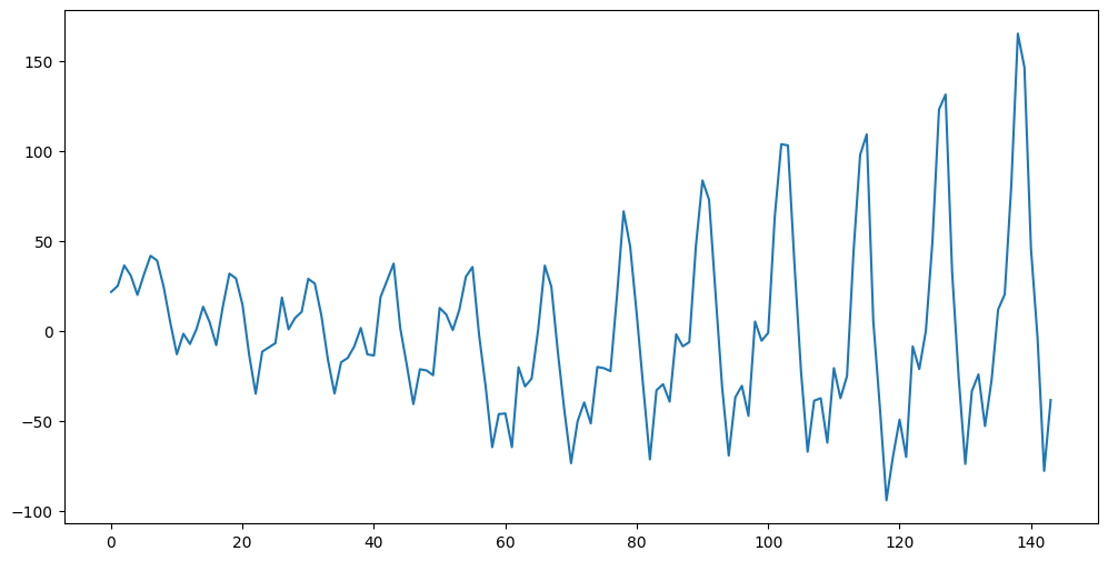
Now let us use LSTM. We will first fit the model to the detrended data, then obtain predictions for the detrended data, and convert these into predictions for the original data.
mu, sig = y_notrend.mean(), y_notrend.std()
y_std = (y_notrend - mu) / sig

X = torch.tensor(y_std[:-1], dtype=torch.float32)
Y = torch.tensor(y_std[1: ], dtype=torch.float32)

X = X.unsqueeze(0).unsqueeze(-1)   # shape (1, seq_len, 1)
Y = Y.unsqueeze(0).unsqueeze(-1)   # shape (1, seq_len, 1)

seq_len = X.size(1)
print(seq_len)
143
class lstm_net(nn.Module):
    def __init__(self, nh):
        super().__init__()
        self.rnn = nn.LSTM(input_size=1, hidden_size=nh,
                           batch_first=True)
        self.fc  = nn.Linear(nh, 1)      # many-to-many

    def forward(self, x, hc=None):
        out, hc = self.rnn(x, hc)        # out: (batch_size, seq_len, hidden_size)
        out     = self.fc(out)           # (batch_size, seq_len, 1)
        return out, hc

torch.manual_seed(0)
np.random.seed(0)

nh = 200
model = lstm_net(nh)
criterion = nn.MSELoss()
opt = torch.optim.Adam(model.parameters(), lr=1e-3)

n_epochs = 1000
for epoch in range(1, n_epochs + 1):
    #model.train()
    opt.zero_grad()
    pred, _ = model(X)           # hidden state auto-reset every epoch
    loss = criterion(pred, Y)
    loss.backward()
    opt.step()

    if epoch % 100 == 0:
        print(f"epoch {epoch:4d}/{n_epochs}  |  loss = {loss.item():.6f}")

n_future = 60
#model.eval()
with torch.no_grad():
    _, hc = model(X)
    preds = np.zeros(n_future, dtype=np.float32)
    last_in = torch.tensor([[y_std[-1]]], dtype=torch.float32)  # (1, 1, 1) after view

    for t in range(n_future):
        out, hc = model(last_in.view(1, 1, 1), hc)              # reuse hidden state
        next_val = out.squeeze().item()
        preds[t] = next_val
        last_in = torch.tensor([[next_val]], dtype=torch.float32)

tme_pred_axis = np.arange(n, n+n_future)
lstm_preds_orig = (preds * sig + mu) + linmod.params[0] + linmod.params[1] * tme_pred_axis

plt.figure(figsize = (12,6))
plt.plot(np.arange(n), y, lw = 2, label = "Data")
plt.plot(tme_pred_axis, lstm_preds_orig, lw = 2, color = "r", label = "Forecast (LSTM)")
plt.xlabel("Time"); plt.ylabel("Data")
plt.title("Airlines Passengers Data and Forecast using LSTM")
plt.legend()
plt.tight_layout()
plt.show()
epoch 100/1000 | loss = 0.133838
epoch 200/1000 | loss = 0.074407
epoch 300/1000 | loss = 0.063738
epoch 400/1000 | loss = 0.053620
epoch 500/1000 | loss = 0.040483
epoch 600/1000 | loss = 0.024853
epoch 700/1000 | loss = 0.014565
epoch 800/1000 | loss = 0.006797
epoch 900/1000 | loss = 0.007944
epoch 1000/1000 | loss = 0.004411