import numpy as np
import pandas as pd
import matplotlib.pyplot as plt
import torch
import torch.nn as nn
import torch.optim as optim
import statsmodels.api as sm
from statsmodels.tsa.ar_model import AutoReg
from statsmodels.tsa.arima.model import ARIMA
The LSTM Unit
Before fitting LSTM models, let us first see how the basic LSTM unit in PyTorcy (nn.LSTM) works (see \url{https://
To create the LSTM unit, we only need to specify the input_size (this is the dimension of ) and the number of hidden units (this is the dimension of ).
lstm_net = nn.LSTM(input_size = 1, hidden_size = 5, batch_first = True) The above code line will create a LSTM unit and will randomly initialize all its parameters. Given a sequence for some (here each needs to be of dimension input_size), the LSTM unit will then use the formulas to compute . It will output as well as .
If we create two sets of input sequences and , then the LSTM unit will use its formulae to output (as well as ) corresponding to , as well as , as well as corresponding to . In general, if we send in input sequences (i.e., batches of input sequences), each sequence having length (and each in each sequence has dimension input_size), the output of the LSTM will correspond to sequences of length (each element of the sequence has dimension equal to hidden_size). The inputs and outputs can therefore both be treated as tensors. The ‘batch_first = True’ in the specification of lstm_net above indicates that the input tensor should have shape (B, T, input_size) and the output tensor will have shape (B, T, hidden_size).
#Let us create an input tensor for lstm_net:
input = torch.randn(1, 10, 1)
#this input has one batch, which is a sequence x_1, \dots, x_10 of length 10. Each x_t is a scalar (input_size = 1).
print(input)

output, (hn, cn) = lstm_net(input)

#output will have shape (1, 10, 5). It is a simply the sequence h_1, \dots, h_10 where each h_t is of dimension hidden_size = 5.
print(output.shape)

print(hn.shape) #h_n is simply the hidden vector h_t corresponding to the last time (here t = 10). You can check that hn is identical to the last element of the output

print(cn.shape) #c_n is the cell state corresponding to the last output

print(output[:, 9, :])
print(hn)
#check that hn and output[:, 9, :] are identical
tensor([[[-0.8748],
[-1.5131],
[ 0.5044],
[-0.3878],
[ 1.0426],
[ 0.7758],
[-2.0535],
[ 1.3216],
[-0.5709],
[-0.1411]]])
torch.Size([1, 10, 5])
torch.Size([1, 1, 5])
torch.Size([1, 1, 5])
tensor([[ 0.0240, -0.1298, 0.1951, -0.0680, 0.1436]],
grad_fn=<SliceBackward0>)
tensor([[[ 0.0240, -0.1298, 0.1951, -0.0680, 0.1436]]],
grad_fn=<StackBackward0>)
The weight matrices as well as , and the biases as well as can be accessed as follows.
print(lstm_net.weight_ih_l0.shape)
print(lstm_net.weight_ih_l0) #this contains the four weight matrices W_{ii}, W_{if}, W_{ig}, W_{io}

print(lstm_net.weight_hh_l0.shape)
print(lstm_net.weight_hh_l0) #this contains the four weight matrices W_{hi}, W_{hf}, W_{hg}, W_{ho}

print(lstm_net.bias_ih_l0.shape)
print(lstm_net.bias_ih_l0)  #this contains  the four biases b_{ii}, b_{if}, b_{ig}, b_{io}

print(lstm_net.bias_hh_l0.shape)
print(lstm_net.bias_hh_l0)  #this contains  the four biases b_{hi}, b_{hf}, b_{hg}, b_{ho}

#0 here refers to the fact that there is a single LSTM layer. Sometimes, it is common to stack multiple LSTM units, in which case there will be weights and biases for each LSTM. We will only deal with a single LSTM layer
torch.Size([20, 1])
Parameter containing:
tensor([[-0.2318],
        [ 0.1864],
        [ 0.2214],
        [ 0.0846],
        [ 0.1032],
        [ 0.1183],
        [-0.4182],
        [ 0.0963],
        [ 0.0765],
        [-0.1803],
        [-0.3270],
        [ 0.3187],
        [-0.1421],
        [ 0.2497],
        [-0.0431],
        [-0.4423],
        [-0.2981],
        [ 0.0622],
        [ 0.1202],
        [-0.3805]], requires_grad=True)
torch.Size([20, 5])
Parameter containing:
tensor([[-0.1067, -0.1284,  0.0910, -0.4090,  0.3202],
        [ 0.3550,  0.0644, -0.3108,  0.2166,  0.2723],
        [-0.1922, -0.1219, -0.2929, -0.4380,  0.2305],
        [-0.3198,  0.2493, -0.3492, -0.0558, -0.0403],
        [-0.0872, -0.1000,  0.3376, -0.1066,  0.2932],
        [-0.4185,  0.3633, -0.2426, -0.2061, -0.2156],
        [-0.2836, -0.1734, -0.2273,  0.0486,  0.3997],
        [-0.3430,  0.1009,  0.1448,  0.1808,  0.0743],
        [-0.0858, -0.0531, -0.2424,  0.1392, -0.2152],
        [-0.2396, -0.0764,  0.3373,  0.2089, -0.1031],
        [-0.4066,  0.0305,  0.2224,  0.3208, -0.2497],
        [ 0.3759, -0.2133, -0.1815, -0.4049,  0.1355],
        [-0.0020, -0.0276, -0.1923,  0.0173, -0.0990],
        [ 0.3280, -0.4143,  0.3849,  0.0693,  0.2058],
        [ 0.0817,  0.0821,  0.2356, -0.1024,  0.3197],
        [ 0.2500, -0.0572, -0.1750, -0.3839, -0.0397],
        [ 0.3731, -0.2695,  0.3761, -0.1600, -0.2923],
        [ 0.2802,  0.3042, -0.2077,  0.2802,  0.0779],
        [-0.1548, -0.2795, -0.3600,  0.2207,  0.0150],
        [-0.4269,  0.0217,  0.1036, -0.1682,  0.1018]], requires_grad=True)
torch.Size([20])
Parameter containing:
tensor([-0.0022,  0.4127,  0.3966, -0.2505, -0.1704, -0.3527, -0.3993, -0.0755,
         0.0578, -0.4365, -0.2093, -0.3626,  0.4391, -0.4461,  0.2969, -0.4436,
        -0.4349, -0.3425, -0.0728, -0.1951], requires_grad=True)
torch.Size([20])
Parameter containing:
tensor([ 0.2023,  0.4403, -0.0639,  0.4350, -0.3475,  0.0915,  0.3100,  0.3265,
        -0.4368, -0.2926,  0.2324,  0.0268, -0.0123,  0.1047,  0.1561,  0.1119,
        -0.2914,  0.1804, -0.3680,  0.0802], requires_grad=True)
The values that we see above for the weights and biases are randomly chosen initial values. Given some data, they will be trained so as to minimize some loss function.
Simulated Dataset One
Consider the following simple dataset.
n = 1500
truelag = 85
rng = np.random.default_rng(seed = 0)
sig_noise = 0.2
eps = rng.normal(loc = 0, scale = sig_noise, size = n)
y_sim = np.full(shape = n, fill_value = -999.0)
y_sim[0:truelag] = np.linspace(-1, 1, truelag)
for i in range(truelag, n):
    y_sim[i] = y_sim[i - truelag]
y_sim = y_sim + eps
plt.figure(figsize = (12, 6))
plt.plot(y_sim)
plt.show()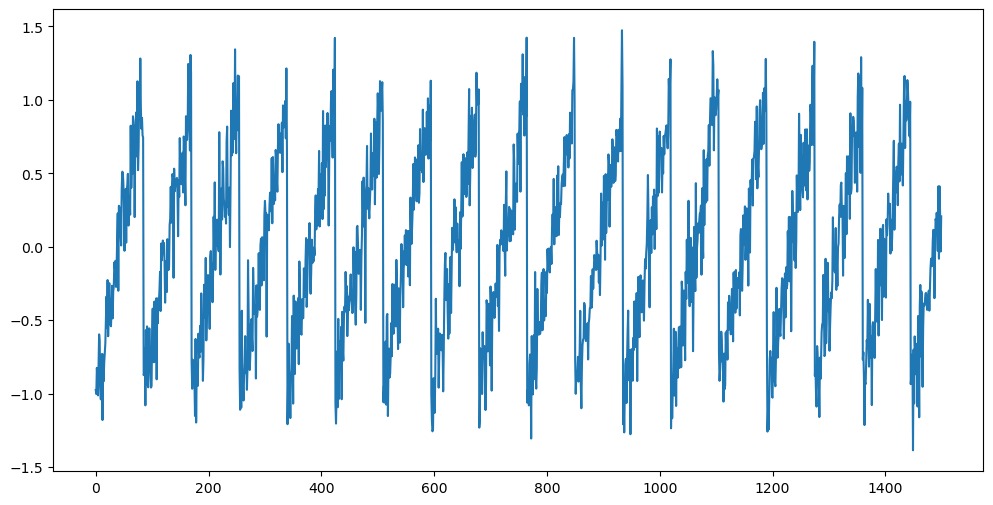
We first fit the AR() model. If is taken to be smaller than the true lag which generated the data, the predictions will be quite poor. But the predictions are quite good when is exactly equal to the true lag.
#Let us fit AR(p) with the truelag
p = truelag
ar = AutoReg(y_sim, lags = p).fit()

n = len(y_sim)
tme = range(1, n+1)
n_future = 1000
tme_future = range(n+1, n+n_future+1)
fcast = ar.get_prediction(start = n, end = n+n_future-1).predicted_mean
plt.figure(figsize = (12, 7))
plt.plot(tme, y_sim, label = 'Data')
plt.plot(tme_future, fcast, label = 'Forecast (AR(p))', color = 'green')
plt.axvline(x=n, color='gray', linestyle='--')
plt.legend()
plt.show()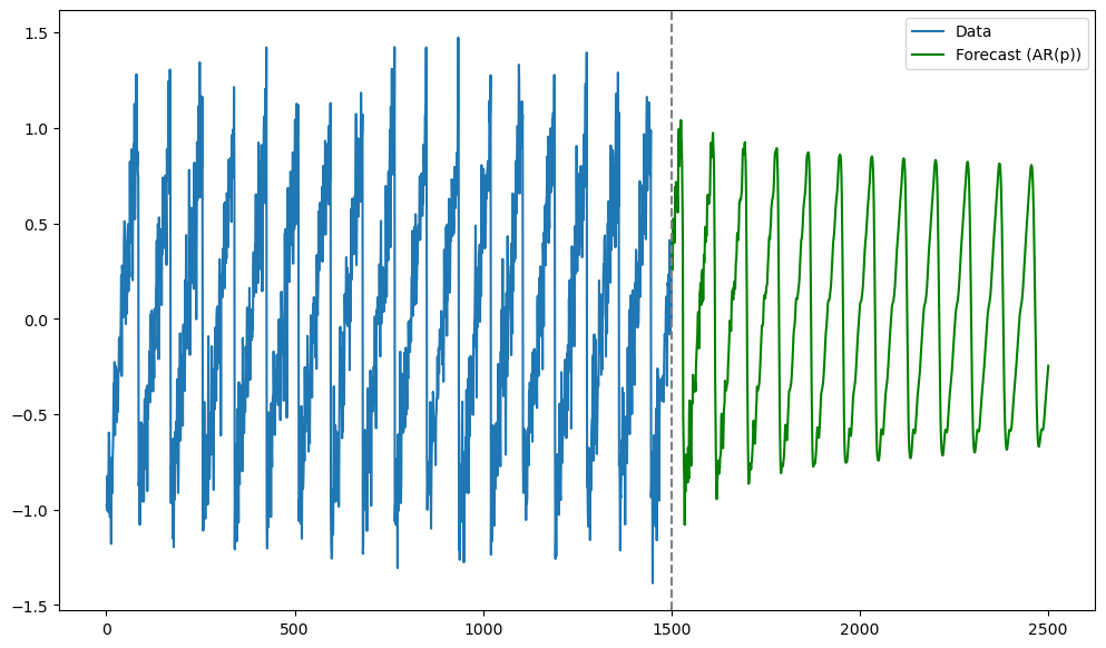
Next we apply LSTM (and RNN). The first step is to create the input and output tensors.
mu, sig = y_sim.mean(), y_sim.std()
y_std = (y_sim - mu) / sig

X = torch.tensor(y_std[:-1], dtype=torch.float32)
Y = torch.tensor(y_std[1: ], dtype=torch.float32)

X = X.unsqueeze(0).unsqueeze(-1)   # shape (1, seq_len, 1)
Y = Y.unsqueeze(0).unsqueeze(-1)   # shape (1, seq_len, 1)

seq_len = X.size(1)
print(seq_len)
1499
We create the LSTM model class below.
class lstm_net(nn.Module):
    def __init__(self, nh):
        super().__init__()
        self.rnn = nn.LSTM(input_size=1, hidden_size=nh,
                           batch_first=True)
        self.fc  = nn.Linear(nh, 1)
    def forward(self, x, hc=None):
        out, hc = self.rnn(x, hc)
        out     = self.fc(out)
        return out, hc

#lstm_net defined above has an LSTM unit followed by a linear unit ('fc' stands for fully-connected) which converts the output of the LSTM to a scalar (this scalar is mu_t in our notation)

torch.manual_seed(0)
np.random.seed(0)

nh = 100
model = lstm_net(nh)
criterion = nn.MSELoss()
opt = torch.optim.Adam(model.parameters(), lr=1e-3)
Training is done as follows.
n_epochs = 1000
for epoch in range(1, n_epochs + 1):
    model.train()
    opt.zero_grad()
    pred, _ = model(X)
    loss = criterion(pred, Y)
    loss.backward()
    opt.step()

    if epoch % 100 == 0:
        print(f"epoch {epoch:4d}/{n_epochs}  |  loss = {loss.item():.6f}")
epoch 100/1000 | loss = 0.238784
epoch 200/1000 | loss = 0.183601
epoch 300/1000 | loss = 0.178046
epoch 400/1000 | loss = 0.165648
epoch 500/1000 | loss = 0.161582
epoch 600/1000 | loss = 0.155341
epoch 700/1000 | loss = 0.151636
epoch 800/1000 | loss = 0.158860
epoch 900/1000 | loss = 0.158528
epoch 1000/1000 | loss = 0.139661
Predictions are obtained as follows.
model.eval()
with torch.no_grad():
    _, hc = model(X)
    preds = np.zeros(n_future, dtype=np.float32)
    last_in = torch.tensor([[y_std[-1]]], dtype=torch.float32)  # (1, 1, 1) after view
    for t in range(n_future):
        out, hc = model(last_in.view(1, 1, 1), hc)              # reuse hidden state
        next_val = out.squeeze().item()
        preds[t] = next_val
        last_in = torch.tensor([[next_val]], dtype=torch.float32)
Predictions are plotted below.
lstm_preds_orig = preds * sig + mu
tme_pred_axis = np.arange(n, n + n_future)

plt.figure(figsize=(12,6))
plt.plot(np.arange(n), y_sim, lw=2, label="Data")
plt.plot(tme_pred_axis, lstm_preds_orig, lw=2, color="r", label="forecast (LSTM)")
plt.xlabel("Time"); plt.ylabel("Data")
for t in range(0, n + n_future, truelag):
    plt.axvline(x=t, linestyle='--', color='gray', linewidth=1)
plt.axhline(y=1, linestyle='--', color='gray', linewidth=1)
plt.axhline(y=-1, linestyle='--', color='gray', linewidth=1)
plt.title("Data and Forecast")
plt.legend()
plt.tight_layout()
plt.show()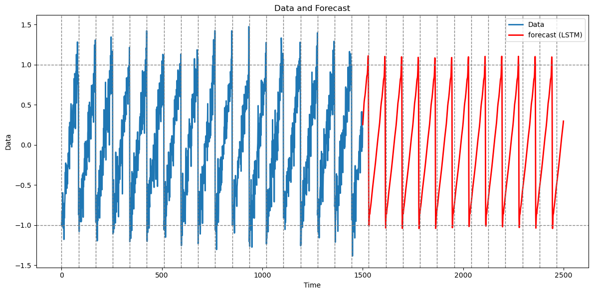
In the code above, the LSTM receives a single stream of length (with batch = 1), so every training step must iterate through 1500 recurrent updates, store all intermediate gate outputs, cell states, and hidden states for back-propagation-through-time, and then sweep backward through those same 1500 steps. The result is a high per-epoch cost--roughly proportional to both in floating-point operations and in memory.
To make the code faster, we can attempt to chunk the original time series into a small number (say 3) of batches of a smaller number (say 450) samples, and then to stack them so that the input tensor is of shape (3, 450, 1). Each forward/backward pass now unrolls only 450 steps (a 3.3 times reduction) and the three batches can even be procesed in parallel along the batch dimension. This combination of a shallower time depth and batching typically leads to a speed up in the code. However, the trade‑off is that the hidden state is implicitly reset at every window boundary, so the model cannot capture dependencies that span more than 450 time steps; for tasks that truly require very long‑range memory, the slower single‑sequence approach is safer.
Below we illustrate this batching idea.
Batching
seq_len_batch = 450
n_batches = (len(y_std) - 1) // seq_len_batch
print(n_batches)

X_batches = []
Y_batches = []
for i in range(n_batches):
    start_idx = i * seq_len_batch
    end_idx = start_idx + seq_len_batch
    X_batches.append(y_std[start_idx : end_idx])
    Y_batches.append(y_std[(start_idx + 1): (end_idx + 1)])

X = torch.tensor(X_batches, dtype = torch.float32).unsqueeze(-1)
Y = torch.tensor(Y_batches, dtype = torch.float32).unsqueeze(-1)

print(X.shape)
print(Y.shape)
3
torch.Size([3, 450, 1])
torch.Size([3, 450, 1])
class lstm_net(nn.Module):
    def __init__(self, nh):
        super().__init__()
        self.rnn = nn.LSTM(input_size=1, hidden_size=nh,
                           batch_first=True)
        self.fc  = nn.Linear(nh, 1)          # many-to-many
    def forward(self, x, hc=None):
        out, hc = self.rnn(x, hc)            # out: (B, T, nh)
        out     = self.fc(out)               # (B, T, 1)
        return out, hc

torch.manual_seed(0)
np.random.seed(0)

nh = 100
model = lstm_net(nh)
criterion = nn.MSELoss()
opt = torch.optim.Adam(model.parameters(), lr=1e-3)
n_epochs = 1000
for epoch in range(1, n_epochs + 1):
model.train()
opt.zero_grad()
pred, _ = model(X)
loss = criterion(pred, Y)
loss.backward()
opt.step()
if epoch % 100 == 0:
print(f"epoch {epoch:4d}/{n_epochs} | loss = {loss.item():.6f}")epoch 100/1000 | loss = 0.235551
epoch 200/1000 | loss = 0.190747
epoch 300/1000 | loss = 0.169411
epoch 400/1000 | loss = 0.158637
epoch 500/1000 | loss = 0.159057
epoch 600/1000 | loss = 0.144519
epoch 700/1000 | loss = 0.151861
epoch 800/1000 | loss = 0.132501
epoch 900/1000 | loss = 0.123780
epoch 1000/1000 | loss = 0.176492
Once the model is trained, I revert back to the previous and (without batching) in order to calculate predictions.
mu, sig = y_sim.mean(), y_sim.std()
y_std = (y_sim - mu) / sig
X = torch.tensor(y_std[:-1], dtype=torch.float32)
Y = torch.tensor(y_std[1: ], dtype=torch.float32)
X = X.unsqueeze(0).unsqueeze(-1) # shape (1, seq_len, 1)
Y = Y.unsqueeze(0).unsqueeze(-1) # shape (1, seq_len, 1)
seq_len = X.size(1)
print(seq_len)
model.eval()
with torch.no_grad():
_, hc = model(X)
preds = np.zeros(n_future, dtype=np.float32)
last_in = torch.tensor([[y_std[-1]]], dtype=torch.float32) # (1, 1, 1) after view
for t in range(n_future):
out, hc = model(last_in.view(1, 1, 1), hc) # reuse hidden state
next_val = out.squeeze().item()
preds[t] = next_val
last_in = torch.tensor([[next_val]], dtype=torch.float32)
lstm_preds_orig_batch = preds * sig + mu
tme_pred_axis = np.arange(n, n + n_future)
plt.figure(figsize=(12,6))
plt.plot(np.arange(n), y_sim, lw=2, label="Data")
plt.plot(tme_pred_axis, lstm_preds_orig, lw=2, color="r", label="forecast (LSTM)")
plt.plot(tme_pred_axis, lstm_preds_orig_batch, lw=2, color="green", label="forecast (LSTM Batch)")
plt.xlabel("Time"); plt.ylabel("Data")
plt.title("Data and Forecast")
for t in range(0, n + n_future, truelag):
plt.axvline(x=t, linestyle='--', color='gray', linewidth=1)
plt.axhline(y=1, linestyle='--', color='gray', linewidth=1)
plt.axhline(y=-1, linestyle='--', color='gray', linewidth=1)
plt.legend()
plt.tight_layout()
plt.show()1499
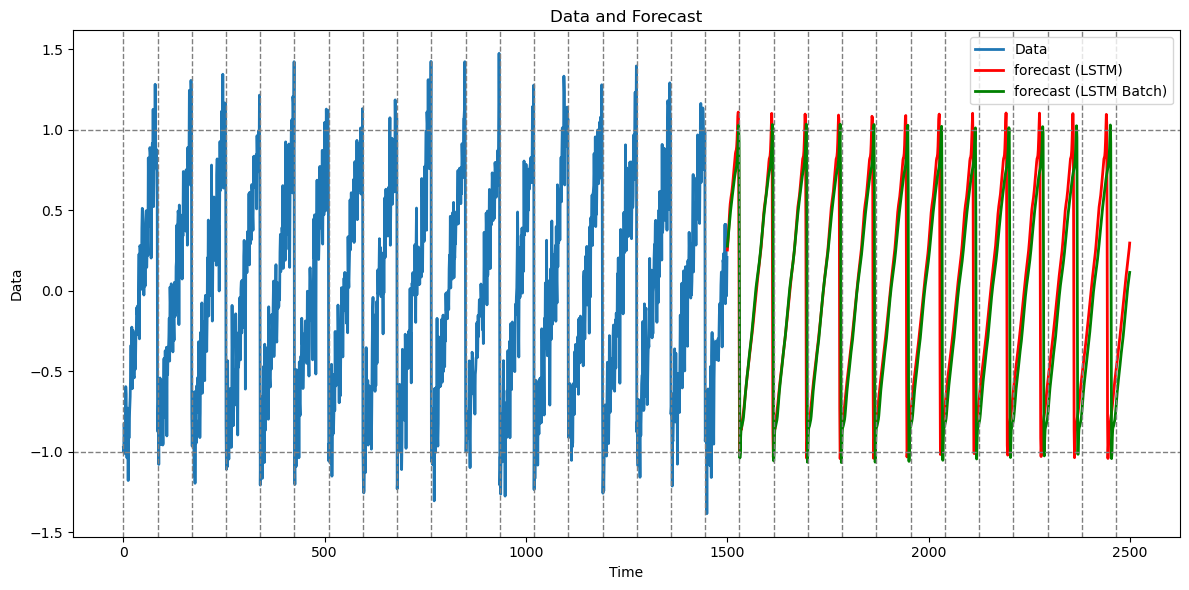
In this example, the predictions with and without batching are nearly identical. However batching makes the code run much faster.
Let us now fit the RNN.
class RNNReg(nn.Module):
def __init__(self, nh):
super().__init__()
self.rnn = nn.RNN(1, nh, nonlinearity="tanh", batch_first=True)
self.fc = nn.Linear(nh, 1)
def forward(self, x, h=None):
out, h = self.rnn(x, h)
return self.fc(out), h
nh = 50
model = RNNReg(nh)
criterion = nn.MSELoss()
opt = torch.optim.Adam(model.parameters(),lr = 1e-3)n_epochs = 1000
for epoch in range(1, n_epochs + 1):
model.train()
opt.zero_grad()
pred, _ = model(X)
loss = criterion(pred, Y)
loss.backward()
opt.step()
if epoch % 100 == 0:
print(f"epoch {epoch:4d}/{n_epochs} | loss = {loss.item():.6f}")epoch 100/1000 | loss = 0.283465
epoch 200/1000 | loss = 0.230474
epoch 300/1000 | loss = 0.199063
epoch 400/1000 | loss = 0.190025
epoch 500/1000 | loss = 0.182842
epoch 600/1000 | loss = 0.219429
epoch 700/1000 | loss = 0.221646
epoch 800/1000 | loss = 0.171874
epoch 900/1000 | loss = 0.169135
epoch 1000/1000 | loss = 0.171711
model.eval()
with torch.no_grad():
_, h = model(X)
preds = np.zeros(n_future, np.float32)
last = torch.tensor([[y_std[-1]]], dtype=torch.float32)
for t in range(n_future):
out, h = model(last.view(1,1,1), h)
preds[t] = out.item()
last = torch.tensor([[preds[t]]], dtype=torch.float32)
rnn_preds_orig = preds * sig + mu
tme_pred_axis = np.arange(n, n + n_future)
plt.figure(figsize=(12,6))
plt.plot(np.arange(n), y_sim, lw=2, label="Data")
plt.plot(tme_pred_axis, lstm_preds_orig, lw=2, color="red", label="forecast (LSTM)")
plt.plot(tme_pred_axis, rnn_preds_orig, lw=2, color="black", label="forecast (RNN)")
for t in range(0, n + n_future, truelag):
plt.axvline(x=t, linestyle='--', color='gray', linewidth=1)
plt.axhline(y=1, linestyle='--', color='gray', linewidth=1)
plt.axhline(y=-1, linestyle='--', color='gray', linewidth=1)
plt.xlabel("Time"); plt.ylabel("Data")
plt.title("Data and Forecast")
plt.legend()
plt.tight_layout()
plt.show()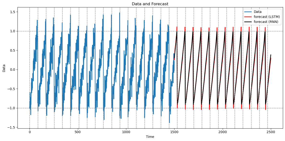
RNN gives predictions that are basically the same as the LSTM predictions.
Simulated Dataset Two
We now make two changes to the first simulation above. We increase the true lag. We also add noise slightly differently (noise is now added to the equation ).
n = 1500
truelag = 344
rng = np.random.default_rng(seed = 0)
sig_noise = 0.2
eps = rng.normal(loc = 0, scale = sig_noise, size = n)
y_sim = np.full(shape = n, fill_value = -999.0)
y_sim[0:truelag] = np.linspace(-1, 1, truelag)
for i in range(truelag, n):
y_sim[i] = y_sim[i - truelag] + eps[i]
#y_sim = y_sim + eps
plt.figure(figsize = (12, 6))
plt.plot(y_sim)
plt.show()
This is a long range prediction problem. In this example, AR() with taken to be the true lag gives very noisy predictions (as shown below)
#Let us fit AR(p)
p = truelag
ar = AutoReg(y_sim, lags = p).fit()
n = len(y_sim)
tme = range(1, n+1)
n_future = 1000
tme_future = range(n+1, n+n_future+1)
fcast = ar.get_prediction(start = n, end = n+n_future-1).predicted_mean
plt.figure(figsize = (12, 7))
plt.plot(tme, y_sim, label = 'Data')
plt.plot(tme_future, fcast, label = 'Forecast (AR(p))', color = 'green')
plt.axvline(x=n, color='gray', linestyle='--')
plt.legend()
plt.show()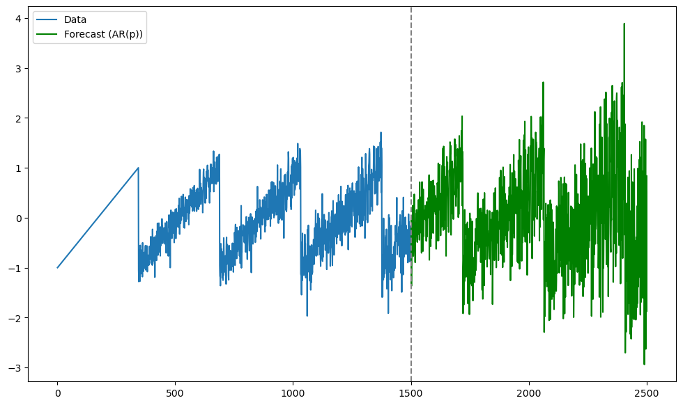
Let us see how the LSTM and RNN do. First we fit LSTM without any batching.
mu, sig = y_sim.mean(), y_sim.std()
y_std = (y_sim - mu) / sig
X = torch.tensor(y_std[:-1], dtype=torch.float32)
Y = torch.tensor(y_std[1: ], dtype=torch.float32)
X = X.unsqueeze(0).unsqueeze(-1) # shape (1, seq_len, 1)
Y = Y.unsqueeze(0).unsqueeze(-1) # shape (1, seq_len, 1)
seq_len = X.size(1)
print(seq_len)1499
class lstm_net(nn.Module):
def __init__(self, nh):
super().__init__()
self.rnn = nn.LSTM(input_size=1, hidden_size=nh,
batch_first=True)
self.fc = nn.Linear(nh, 1)
def forward(self, x, hc=None):
out, hc = self.rnn(x, hc)
out = self.fc(out)
return out, hc
torch.manual_seed(0)
np.random.seed(0)
nh = 100
model = lstm_net(nh)
criterion = nn.MSELoss()
opt = torch.optim.Adam(model.parameters(), lr=1e-3)
n_epochs = 1000
for epoch in range(1, n_epochs + 1):
    model.train()
    opt.zero_grad()
    pred, _ = model(X)
    loss = criterion(pred, Y)
    loss.backward()
    opt.step()

    if epoch % 100 == 0:
        print(f"epoch {epoch:4d}/{n_epochs}  |  loss = {loss.item():.6f}")
epoch 100/1000 | loss = 0.234757
epoch 200/1000 | loss = 0.207985
epoch 300/1000 | loss = 0.206311
epoch 400/1000 | loss = 0.195433
epoch 500/1000 | loss = 0.189044
epoch 600/1000 | loss = 0.179978
epoch 700/1000 | loss = 0.173883
epoch 800/1000 | loss = 0.174173
epoch 900/1000 | loss = 0.168488
epoch 1000/1000 | loss = 0.162189
model.eval()
with torch.no_grad():
_, hc = model(X)
preds = np.zeros(n_future, dtype=np.float32)
last_in = torch.tensor([[y_std[-1]]], dtype=torch.float32) # (1, 1, 1) after view
for t in range(n_future):
out, hc = model(last_in.view(1, 1, 1), hc) # reuse hidden state
next_val = out.squeeze().item()
preds[t] = next_val
last_in = torch.tensor([[next_val]], dtype=torch.float32)lstm_preds_orig = preds * sig + mu
tme_pred_axis = np.arange(n, n + n_future)
plt.figure(figsize=(12,6))
plt.plot(np.arange(n), y_sim, lw=2, label="Data")
plt.plot(tme_pred_axis, lstm_preds_orig, lw=2, color="r", label="forecast (LSTM)")
plt.xlabel("Time"); plt.ylabel("Data")
for t in range(0, n + n_future, truelag):
plt.axvline(x=t, linestyle='--', color='gray', linewidth=1)
plt.axhline(y=1, linestyle='--', color='gray', linewidth=1)
plt.axhline(y=-1, linestyle='--', color='gray', linewidth=1)
plt.title("Data and Forecast")
plt.legend()
plt.tight_layout()
plt.show()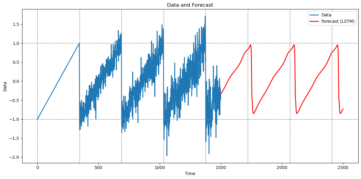
The predictions are decent. Note that the nature of the predictions (which seem quite clean) is quite different from the predictions given by the AR model (these were very noisy).
Now let us apply batching.
seq_len_batch = 650
n_batches = (len(y_std) - 1) // seq_len_batch
print(n_batches)
X_batches = []
Y_batches = []
for i in range(n_batches):
start_idx = i * seq_len_batch
end_idx = start_idx + seq_len_batch
X_batches.append(y_std[start_idx : end_idx])
Y_batches.append(y_std[(start_idx + 1): (end_idx + 1)])
X = torch.tensor(X_batches, dtype = torch.float32).unsqueeze(-1)
Y = torch.tensor(Y_batches, dtype = torch.float32).unsqueeze(-1)
print(X.shape)
print(Y.shape)
2
torch.Size([2, 650, 1])
torch.Size([2, 650, 1])
class lstm_net(nn.Module):
def __init__(self, nh):
super().__init__()
self.rnn = nn.LSTM(input_size=1, hidden_size=nh,
batch_first=True)
self.fc = nn.Linear(nh, 1)
def forward(self, x, hc=None):
out, hc = self.rnn(x, hc)
out = self.fc(out)
return out, hc
torch.manual_seed(0)
np.random.seed(0)
nh = 100
model = lstm_net(nh)
criterion = nn.MSELoss()
opt = torch.optim.Adam(model.parameters(), lr=1e-3)n_epochs = 1000
for epoch in range(1, n_epochs + 1):
model.train()
opt.zero_grad()
pred, _ = model(X)
loss = criterion(pred, Y)
loss.backward()
opt.step()
if epoch % 100 == 0:
print(f"epoch {epoch:4d}/{n_epochs} | loss = {loss.item():.6f}")epoch 100/1000 | loss = 0.196386
epoch 200/1000 | loss = 0.172178
epoch 300/1000 | loss = 0.158832
epoch 400/1000 | loss = 0.158074
epoch 500/1000 | loss = 0.177489
epoch 600/1000 | loss = 0.157444
epoch 700/1000 | loss = 0.150786
epoch 800/1000 | loss = 0.147682
epoch 900/1000 | loss = 0.143554
epoch 1000/1000 | loss = 0.136835
mu, sig = y_sim.mean(), y_sim.std()
y_std = (y_sim - mu) / sig

X = torch.tensor(y_std[:-1], dtype=torch.float32)
Y = torch.tensor(y_std[1: ], dtype=torch.float32)

X = X.unsqueeze(0).unsqueeze(-1)   # shape (1, seq_len, 1)
Y = Y.unsqueeze(0).unsqueeze(-1)   # shape (1, seq_len, 1)

seq_len = X.size(1)
print(seq_len)

model.eval()
with torch.no_grad():
    _, hc = model(X)
    preds = np.zeros(n_future, dtype=np.float32)
    last_in = torch.tensor([[y_std[-1]]], dtype=torch.float32)  # (1, 1, 1) after view
    for t in range(n_future):
        out, hc = model(last_in.view(1, 1, 1), hc)              # reuse hidden state
        next_val = out.squeeze().item()
        preds[t] = next_val
        last_in = torch.tensor([[next_val]], dtype=torch.float32)

lstm_preds_orig_batch = preds * sig + mu
tme_pred_axis = np.arange(n, n + n_future)

plt.figure(figsize=(12,6))
plt.plot(np.arange(n), y_sim, lw=2, label="Data")
plt.plot(tme_pred_axis, lstm_preds_orig, lw=2, color="r", label="forecast (LSTM)")
plt.plot(tme_pred_axis, lstm_preds_orig_batch, lw=2, color="green", label="forecast (LSTM Batch)")
plt.xlabel("Time"); plt.ylabel("Data")
plt.title("Data and Forecast")
for t in range(0, n + n_future, truelag):
    plt.axvline(x=t, linestyle='--', color='gray', linewidth=1)
plt.axhline(y=1, linestyle='--', color='gray', linewidth=1)
plt.axhline(y=-1, linestyle='--', color='gray', linewidth=1)
plt.legend()
plt.tight_layout()
plt.show()
1499
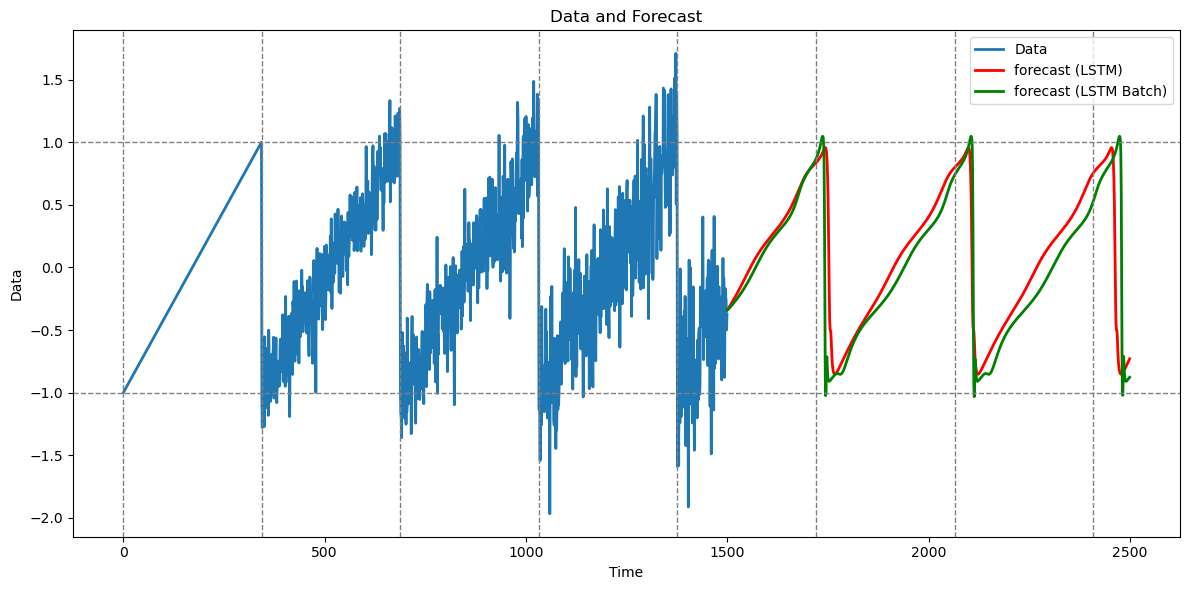
The predictions with and without batching are similar (I am using sequence length equaling 650 here; for different values of this parameter, the predictions seem different from the full-sequence predictions).
RNN does not seem to work for this predictions as shown below (this is because of the lack of ability to capture long range dependencies).
class RNNReg(nn.Module):
def __init__(self, nh):
super().__init__()
self.rnn = nn.RNN(1, nh, nonlinearity="tanh", batch_first=True)
self.fc = nn.Linear(nh, 1)
def forward(self, x, h=None):
out, h = self.rnn(x, h)
return self.fc(out), h
nh = 50 #I could not find any value of nh for which the RNN is giving good predictions for this data
model = RNNReg(nh)
criterion = nn.MSELoss()
opt = torch.optim.Adam(model.parameters(),lr = 1e-3)n_epochs = 1000
for epoch in range(1, n_epochs + 1):
model.train()
opt.zero_grad()
pred, _ = model(X)
loss = criterion(pred, Y)
loss.backward()
opt.step()
if epoch % 100 == 0:
print(f"epoch {epoch:4d}/{n_epochs} | loss = {loss.item():.6f}")epoch 100/1000 | loss = 0.234295
epoch 200/1000 | loss = 0.228924
epoch 300/1000 | loss = 0.224068
epoch 400/1000 | loss = 0.208632
epoch 500/1000 | loss = 0.220152
epoch 600/1000 | loss = 0.195136
epoch 700/1000 | loss = 0.190942
epoch 800/1000 | loss = 0.219482
epoch 900/1000 | loss = 0.197227
epoch 1000/1000 | loss = 0.197343
model.eval()
with torch.no_grad():
_, h = model(X)
preds = np.zeros(n_future, np.float32)
last = torch.tensor([[y_std[-1]]], dtype=torch.float32)
for t in range(n_future):
out, h = model(last.view(1,1,1), h)
preds[t] = out.item()
last = torch.tensor([[preds[t]]], dtype=torch.float32)
rnn_preds_orig = preds * sig + mu
tme_pred_axis = np.arange(n, n + n_future)
plt.figure(figsize=(12,6))
plt.plot(np.arange(n), y_sim, lw=2, label="Data")
plt.plot(tme_pred_axis, lstm_preds_orig, lw=2, color="red", label="forecast (LSTM)")
plt.plot(tme_pred_axis, rnn_preds_orig, lw=2, color="black", label="forecast (RNN)")
for t in range(0, n + n_future, truelag):
plt.axvline(x=t, linestyle='--', color='gray', linewidth=1)
plt.axhline(y=1, linestyle='--', color='gray', linewidth=1)
plt.axhline(y=-1, linestyle='--', color='gray', linewidth=1)
plt.xlabel("Time"); plt.ylabel("Data")
plt.title("Data and Forecast")
plt.legend()
plt.tight_layout()
plt.show()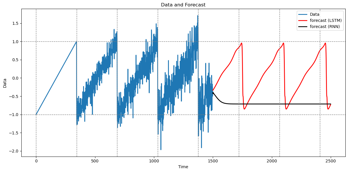
Sunspots Data
Below we apply LSTM, RNN and GRU to obtain predictions for the sunspots dataset.
sunspots = pd.read_csv('SN_y_tot_V2.0.csv', header = None, sep = ';')
print(sunspots.head())
y = sunspots.iloc[:,1].values
n = len(y)
plt.figure(figsize = (12, 6))
plt.plot(y)
plt.show()
print(n)
n_future = 300 0 1 2 3 4
0 1700.5 8.3 -1.0 -1 1
1 1701.5 18.3 -1.0 -1 1
2 1702.5 26.7 -1.0 -1 1
3 1703.5 38.3 -1.0 -1 1
4 1704.5 60.0 -1.0 -1 1
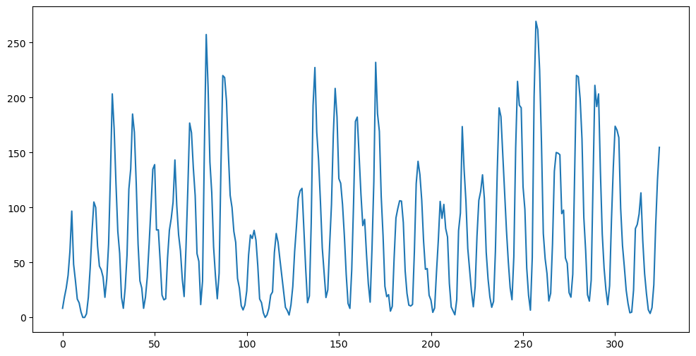
325
Because the data size is not very large, we do not use any batching and directly apply the models on the full sequence. First we prepare and .
mu, sig = y.mean(), y.std()
y_std = (y - mu) / sig
X = torch.tensor(y_std[:-1], dtype=torch.float32)
Y = torch.tensor(y_std[1: ], dtype=torch.float32)
X = X.unsqueeze(0).unsqueeze(-1) # shape (1, seq_len, 1)
Y = Y.unsqueeze(0).unsqueeze(-1) # shape (1, seq_len, 1)
seq_len = X.size(1)
print(seq_len)324
We fit LSTM with the number of hidden units equaling 200.
LSTM for Sunspots
class lstm_net(nn.Module):
def __init__(self, nh):
super().__init__()
self.rnn = nn.LSTM(input_size=1, hidden_size=nh,
batch_first=True)
self.fc = nn.Linear(nh, 1)
def forward(self, x, hc=None):
out, hc = self.rnn(x, hc)
out = self.fc(out)
return out, hc
torch.manual_seed(0)
np.random.seed(0)
nh = 200
model = lstm_net(nh)
criterion = nn.MSELoss()
opt = torch.optim.Adam(model.parameters(), lr=1e-3)
n_epochs = 1000
for epoch in range(1, n_epochs + 1):
    model.train()
    opt.zero_grad()
    pred, _ = model(X)
    loss = criterion(pred, Y)
    loss.backward()
    opt.step()

    if epoch % 100 == 0:
        print(f"epoch {epoch:4d}/{n_epochs}  |  loss = {loss.item():.6f}")
epoch 100/1000 | loss = 0.126732
epoch 200/1000 | loss = 0.059227
epoch 300/1000 | loss = 0.040492
epoch 400/1000 | loss = 0.015958
epoch 500/1000 | loss = 0.016379
epoch 600/1000 | loss = 0.012615
epoch 700/1000 | loss = 0.005350
epoch 800/1000 | loss = 0.005683
epoch 900/1000 | loss = 0.001991
epoch 1000/1000 | loss = 0.001579
model.eval()
with torch.no_grad():
_, hc = model(X)
preds = np.zeros(n_future, dtype=np.float32)
last_in = torch.tensor([[y_std[-1]]], dtype=torch.float32) # (1, 1, 1) after view
for t in range(n_future):
out, hc = model(last_in.view(1, 1, 1), hc) # reuse hidden state
next_val = out.squeeze().item()
preds[t] = next_val
last_in = torch.tensor([[next_val]], dtype=torch.float32)lstm_preds_orig = preds * sig + mu
tme_pred_axis = np.arange(n, n + n_future)
plt.figure(figsize=(12,6))
plt.plot(np.arange(n), y, lw=2, label="Data")
plt.plot(tme_pred_axis, lstm_preds_orig, lw=2, color="r", label="forecast (LSTM)")
plt.xlabel("Time"); plt.ylabel("Data")
plt.title("Data and Forecast")
plt.legend()
plt.tight_layout()
plt.show()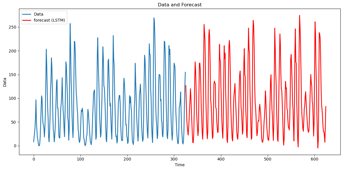
The predictions for the LSTM look quite realistic. They are quite different in characteristic from the predictions generated by an AR() model (the AR() predictions oscillate for a short while before settling to a constant value; in contrast, the LSTM predictions seem to oscillate well into the future in a way that is visually similar to the true dataset).
RNN for Sunspots
Next we apply the RNN (again with 200 hidden units).
torch.manual_seed(0)
np.random.seed(0)
nh = 200
class RNNReg(nn.Module):
def __init__(self):
super().__init__()
self.rnn = nn.RNN(1, nh, nonlinearity="tanh", batch_first=True)
self.fc = nn.Linear(nh, 1)
def forward(self, x, h=None):
out, h = self.rnn(x, h)
return self.fc(out), h
model = RNNReg()
opt = torch.optim.Adam(model.parameters(), lr=1e-3)
lossf = nn.MSELoss()
for epoch in range(1000):
opt.zero_grad()
pred,_ = model(X)
loss = lossf(pred, Y)
loss.backward(); opt.step()
if epoch % 100 == 0:
print(f"epoch {epoch:4d}/{n_epochs} | loss = {loss.item():.6f}")epoch 0/1000 | loss = 1.003679
epoch 100/1000 | loss = 0.141562
epoch 200/1000 | loss = 0.082867
epoch 300/1000 | loss = 0.056757
epoch 400/1000 | loss = 0.047312
epoch 500/1000 | loss = 0.025869
epoch 600/1000 | loss = 0.014358
epoch 700/1000 | loss = 0.008335
epoch 800/1000 | loss = 0.133992
epoch 900/1000 | loss = 0.089119
model.eval()
with torch.no_grad():
    _, h = model(X)
    preds = np.zeros(n_future, np.float32)
    last  = torch.tensor([[y_std[-1]]], dtype=torch.float32)
    for t in range(n_future):
        out, h = model(last.view(1,1,1), h)
        preds[t] = out.item()
        last = torch.tensor([[preds[t]]], dtype=torch.float32)
rnn_preds_orig = preds*sig + mu
tme_pred_axis = np.arange(n, n + n_future)
plt.figure(figsize=(12,6))
plt.plot(np.arange(n), y, lw=2, label="Data")
plt.plot(tme_pred_axis, rnn_preds_orig, lw=2, color="r", label="forecast (RNN)")
plt.xlabel("Time"); plt.ylabel("Data")
plt.title("Data and Forecast")
plt.legend()
plt.tight_layout()
plt.show()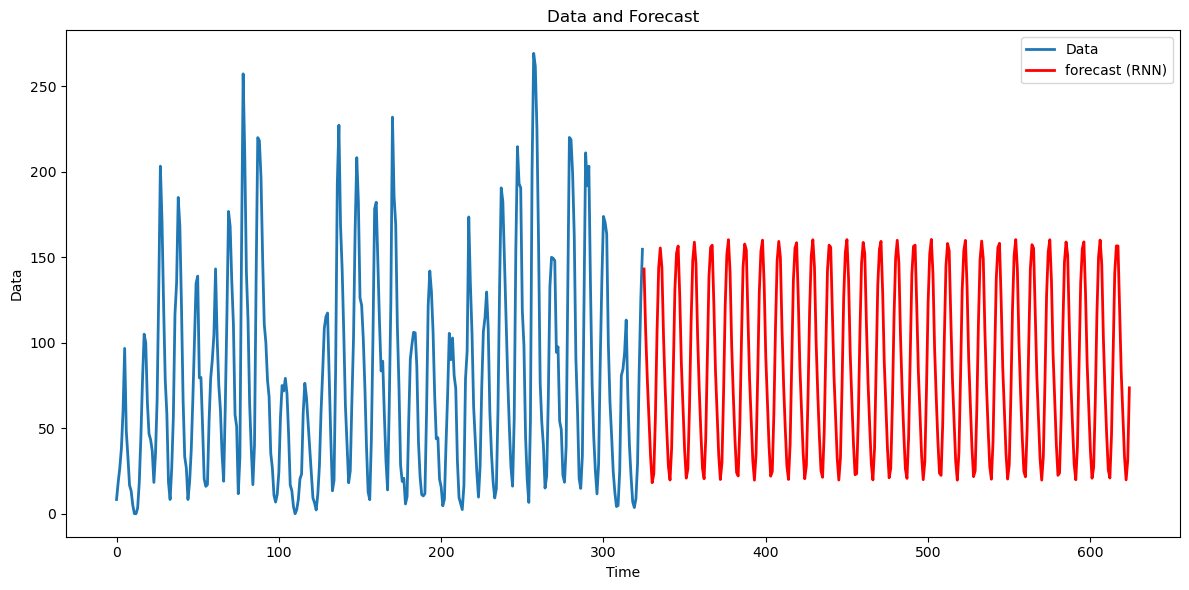
These predictions do not appear as realistic as the LSTM forecasts.
GRU for Sunspots
Below we fit the GRU again with 200 hidden units. The code works in exactly the same way as LSTM and RNN.
torch.manual_seed(0)
np.random.seed(0)

nh = 200
class GRUReg(nn.Module):
    def __init__(self):
        super().__init__()
        self.gru = nn.GRU(1, nh, batch_first=True)
        self.fc  = nn.Linear(nh,1)
    def forward(self,x,h=None):
        out,h = self.gru(x,h)
        return self.fc(out),h
model = GRUReg()
opt = torch.optim.Adam(model.parameters(), lr=1e-3)
lossf = nn.MSELoss()
for epoch in range(1000):
opt.zero_grad()
pred,_ = model(X)
loss = lossf(pred, Y)
loss.backward(); opt.step()
if epoch % 100 == 0:
print(f"epoch {epoch:4d}/{n_epochs} | loss = {loss.item():.6f}")epoch 0/1000 | loss = 1.034648
epoch 100/1000 | loss = 0.124171
epoch 200/1000 | loss = 0.071740
epoch 300/1000 | loss = 0.042880
epoch 400/1000 | loss = 0.033138
epoch 500/1000 | loss = 0.068680
epoch 600/1000 | loss = 0.018391
epoch 700/1000 | loss = 0.074656
epoch 800/1000 | loss = 0.030435
epoch 900/1000 | loss = 0.017239
model.eval()
with torch.no_grad():
    _,h = model(X)
    preds = np.zeros(n_future,np.float32)
    last  = torch.tensor([[y_std[-1]]], dtype=torch.float32)
    for t in range(n_future):
        out,h = model(last.view(1,1,1),h)
        preds[t]=out.item()
        last = torch.tensor([[preds[t]]], dtype=torch.float32)

gru_preds_orig = preds*sig+mu
plt.figure(figsize=(12,6))
plt.plot(np.arange(len(y)),y,lw=2,label="Data")
plt.plot(np.arange(len(y),len(y)+n_future),gru_preds_orig, lw=2,label="Forecast (GRU)",color="orange")
plt.legend()
plt.title("Data and Forecast"); plt.legend(); plt.tight_layout(); plt.show()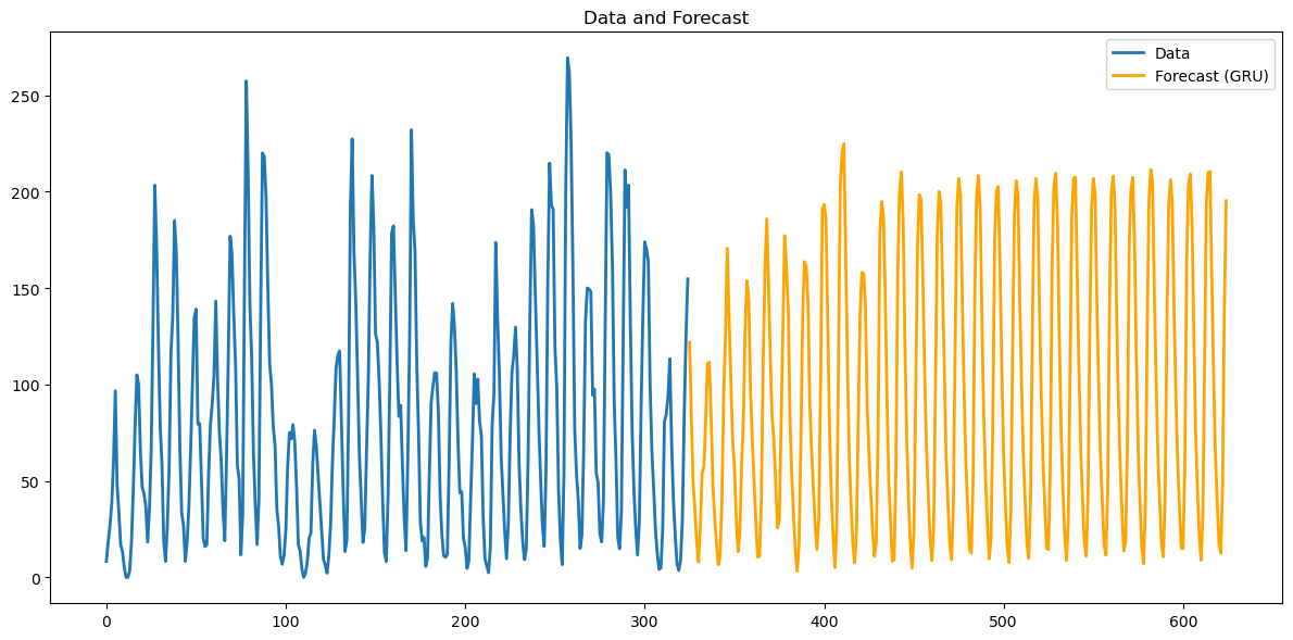
Again the predictions do not look as realistic as those produced by the LSTM.