import numpy as np
import pandas as pd
import matplotlib.pyplot as plt
import statsmodels.api as sm
from statsmodels.tsa.ar_model import AutoReg
Fitting AR(2) to the sunspots dataset
sunspots = pd.read_csv('SN_y_tot_V2.0.csv', header = None, sep = ';')
y = sunspots.iloc[:,1].values
n = len(y)
plt.figure(figsize = (12, 6))
plt.plot(y)
plt.show()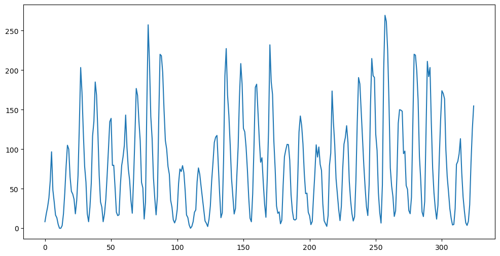
To fit an AR(p) model, we can use the function AutoReg from statsmodels. This implements the conditional MLE method, and gives frequentist standard errors based on the z-score.
armod_sm = AutoReg(y, lags = 2, trend = 'c').fit()
print(armod_sm.summary())
AutoReg Model Results
==============================================================================
Dep. Variable: y No. Observations: 325
Model: AutoReg(2) Log Likelihood -1505.524
Method: Conditional MLE S.D. of innovations 25.588
Date: Tue, 01 Apr 2025 AIC 3019.048
Time: 23:13:59 BIC 3034.159
Sample: 2 HQIC 3025.080
325
==============================================================================
coef std err z P>|z| [0.025 0.975]
------------------------------------------------------------------------------
const 24.4561 2.372 10.308 0.000 19.806 29.106
y.L1 1.3880 0.040 34.685 0.000 1.310 1.466
y.L2 -0.6965 0.040 -17.423 0.000 -0.775 -0.618
Roots
=============================================================================
Real Imaginary Modulus Frequency
-----------------------------------------------------------------------------
AR.1 0.9965 -0.6655j 1.1983 -0.0937
AR.2 0.9965 +0.6655j 1.1983 0.0937
-----------------------------------------------------------------------------
Alternatively, one can simply create and and run the usual OLS. This inference method is also valid and can be seen as the result of Bayesian analysis.
p = 2
n = len(y)
yreg = y[p:] #these are the response values in the autoregression
Xmat = np.ones((n-p, 1)) #this will be the design matrix (X) in the autoregression
for j in range(1, p+1):
    col = y[p-j : n-j].reshape(-1, 1)
    Xmat = np.column_stack([Xmat, col])

armod = sm.OLS(yreg, Xmat).fit()
print(armod.params)
print(armod.summary())
sighat = np.sqrt(np.mean(armod.resid ** 2)) #note that this mean is taken over n-p observations
resdf = n - 2*p - 1
sigols = np.sqrt((np.sum(armod.resid ** 2))/resdf)
print(sighat, sigols)
[24.45610705 1.38803272 -0.69646032]
OLS Regression Results
==============================================================================
Dep. Variable: y R-squared: 0.829
Model: OLS Adj. R-squared: 0.828
Method: Least Squares F-statistic: 774.7
Date: Tue, 01 Apr 2025 Prob (F-statistic): 2.25e-123
Time: 23:14:00 Log-Likelihood: -1505.5
No. Observations: 323 AIC: 3017.
Df Residuals: 320 BIC: 3028.
Df Model: 2
Covariance Type: nonrobust
==============================================================================
coef std err t P>|t| [0.025 0.975]
------------------------------------------------------------------------------
const 24.4561 2.384 10.260 0.000 19.767 29.146
x1 1.3880 0.040 34.524 0.000 1.309 1.467
x2 -0.6965 0.040 -17.342 0.000 -0.775 -0.617
==============================================================================
Omnibus: 33.173 Durbin-Watson: 2.200
Prob(Omnibus): 0.000 Jarque-Bera (JB): 50.565
Skew: 0.663 Prob(JB): 1.05e-11
Kurtosis: 4.414 Cond. No. 231.
==============================================================================
Notes:
[1] Standard Errors assume that the covariance matrix of the errors is correctly specified.
25.588082517109108 25.70774684491223
Here are some observations comparing the above two outputs:
- The parameter estimates are exactly the same.
- The regression summary gives t-scores corresponding to each parameter estimate while the AutoReg summary only gives z-scores
- The standard errors are slightly different.
The standard errors given by the regression summary correspond to the square roots of the diagonal entries of:
while the standard errors reported by AutoReg summary correspond to the square roots of the diagonal entries of:
covmat = (sighat ** 2) * np.linalg.inv(np.dot(Xmat.T, Xmat))
covmat_ols = (sigols ** 2) * np.linalg.inv(np.dot(Xmat.T, Xmat))
print(np.sqrt(np.diag(covmat)))
print(np.sqrt(np.diag(covmat_ols)))
print(armod_sm.bse)
print(armod.bse)
[2.37245465 0.04001781 0.03997354]
[2.38354959 0.04020495 0.04016048]
[2.37245465 0.04001781 0.03997354]
[2.38354959 0.04020495 0.04016048]
Point predictions for future observations can be obtained by running the recursions discussed in class. One can also obtain predictions from the AutoReg object. The following code verifies that both these prediction methods lead to the same output.
#Predictions
k = 100
yhat = np.concatenate([y, np.full(k, -9999)]) #extend data by k placeholder values
phi_vals = armod.params
for i in range(1, k+1):
    ans = phi_vals[0]
    for j in range(1, p+1):
        ans += phi_vals[j] * yhat[n+i-j-1]
    yhat[n+i-1] = ans
predvalues = yhat[n:]

#Predictions using Autoreg:
predvalues_sm = armod_sm.predict(start = n, end = n+k-1)

#Check that both predictions are identical:
print(np.column_stack([predvalues, predvalues_sm]))
[[151.77899784 151.77899784]
[127.38790987 127.38790987]
[ 95.56664388 95.56664388]
[ 68.38511059 68.38511059]
[ 52.81850228 52.81850228]
[ 50.14240008 50.14240008]
[ 57.26940772 57.26940772]
[ 69.0257265 69.0257265 ]
[ 80.38020354 80.38020354]
[ 87.9527796 87.9527796 ]
[ 90.55582018 90.55582018]
[ 88.89492689 88.89492689]
[ 84.7766382 84.7766382 ]
[ 80.21706503 80.21706503]
[ 76.75645296 76.75645296]
[ 75.128572 75.128572 ]
[ 75.27919896 75.27919896]
[ 76.6220286 76.6220286 ]
[ 78.38101438 78.38101438]
[ 79.88731663 79.88731663]
[ 80.75304962 80.75304962]
[ 80.90563559 80.90563559]
[ 80.51448123 80.51448123]
[ 79.86527611 79.86527611]
[ 79.23658165 79.23658165]
[ 78.81607878 78.81607878]
[ 78.67026779 78.67026779]
[ 78.76074092 78.76074092]
[ 78.98787216 78.98787216]
[ 79.24012681 79.24012681]
[ 79.43207661 79.43207661]
[ 79.52282387 79.52282387]
[ 79.51509861 79.51509861]
[ 79.44117383 79.44117383]
[ 79.34394415 79.34394415]
[ 79.26047186 79.26047186]
[ 79.2123262 79.2123262 ]
[ 79.20363358 79.20363358]
[ 79.22509949 79.22509949]
[ 79.26094894 79.26094894]
[ 79.29575899 79.29575899]
[ 79.31910876 79.31910876]
[ 79.32727519 79.32727519]
[ 79.32234827 79.32234827]
[ 79.30982195 79.30982195]
[ 79.29586641 79.29586641]
[ 79.28521975 79.28521975]
[ 79.28016132 79.28016132]
[ 79.28055503 79.28055503]
[ 79.2846245 79.2846245 ]
[ 79.28999886 79.28999886]
[ 79.29462443 79.29462443]
[ 79.29730183 79.29730183]
[ 79.29779663 79.29779663]
[ 79.29661873 79.29661873]
[ 79.29463915 79.29463915]
[ 79.29271179 79.29271179]
[ 79.29141526 79.29141526]
[ 79.29095795 79.29095795]
[ 79.29122618 79.29122618]
[ 79.29191698 79.29191698]
[ 79.29268904 79.29268904]
[ 79.29327955 79.29327955]
[ 79.2935615 79.2935615 ]
[ 79.29354158 79.29354158]
[ 79.29331757 79.29331757]
[ 79.29302051 79.29302051]
[ 79.29276419 79.29276419]
[ 79.29261531 79.29261531]
[ 79.29258716 79.29258716]
[ 79.29265179 79.29265179]
[ 79.2927611 79.2927611 ]
[ 79.29286781 79.29286781]
[ 79.2929398 79.2929398 ]
[ 79.29296541 79.29296541]
[ 79.29295081 79.29295081]
[ 79.29291272 79.29291272]
[ 79.29287 79.29287 ]
[ 79.29283725 79.29283725]
[ 79.29282154 79.29282154]
[ 79.29282254 79.29282254]
[ 79.29283487 79.29283487]
[ 79.29285129 79.29285129]
[ 79.29286549 79.29286549]
[ 79.29287377 79.29287377]
[ 79.29287537 79.29287537]
[ 79.29287182 79.29287182]
[ 79.29286579 79.29286579]
[ 79.29285988 79.29285988]
[ 79.29285588 79.29285588]
[ 79.29285445 79.29285445]
[ 79.29285524 79.29285524]
[ 79.29285734 79.29285734]
[ 79.29285971 79.29285971]
[ 79.29286152 79.29286152]
[ 79.2928624 79.2928624 ]
[ 79.29286235 79.29286235]
[ 79.29286167 79.29286167]
[ 79.29286076 79.29286076]
[ 79.29285998 79.29285998]]
DATASET TWO
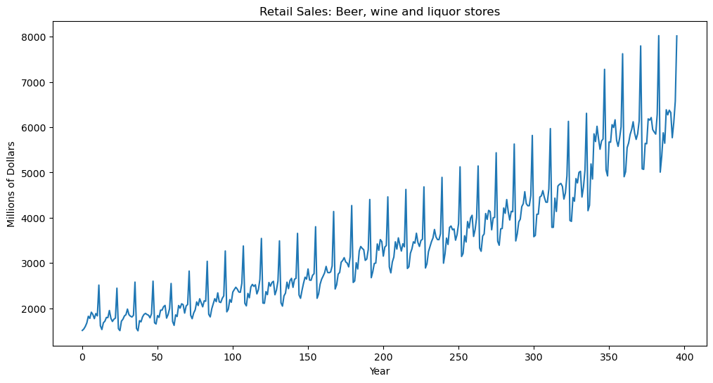
#The following is FRED data on retail sales (in millions of dollars) for beer, wine and liquor stores (https://fred.stlouisfed.org/series/MRTSSM4453USN)
beersales = pd.read_csv('MRTSSM4453USN_March2025.csv')
print(beersales.head())
y = beersales['MRTSSM4453USN'].to_numpy()
n = len(y)
plt.figure(figsize = (12, 6))
plt.plot(y)
plt.xlabel('Year')
plt.ylabel('Millions of Dollars')
plt.title('Retail Sales: Beer, wine and liquor stores')
plt.show()
observation_date MRTSSM4453USN
0 1992-01-01 1509
1 1992-02-01 1541
2 1992-03-01 1597
3 1992-04-01 1675
4 1992-05-01 1822
p = 24
armod_sm = AutoReg(y, lags = p, trend = 'c').fit()
print(armod_sm.summary())
AutoReg Model Results
==============================================================================
Dep. Variable: y No. Observations: 396
Model: AutoReg(24) Log Likelihood -2236.965
Method: Conditional MLE S.D. of innovations 98.930
Date: Tue, 01 Apr 2025 AIC 4525.930
Time: 23:15:15 BIC 4627.821
Sample: 24 HQIC 4566.394
396
==============================================================================
coef std err z P>|z| [0.025 0.975]
------------------------------------------------------------------------------
const 1.5601 15.014 0.104 0.917 -27.866 30.987
y.L1 0.2321 0.051 4.576 0.000 0.133 0.332
y.L2 0.3560 0.052 6.828 0.000 0.254 0.458
y.L3 0.4103 0.055 7.431 0.000 0.302 0.519
y.L4 -0.0642 0.058 -1.105 0.269 -0.178 0.050
y.L5 -0.0558 0.058 -0.955 0.339 -0.170 0.059
y.L6 -0.0576 0.058 -0.985 0.324 -0.172 0.057
y.L7 -0.0500 0.059 -0.854 0.393 -0.165 0.065
y.L8 0.0190 0.059 0.325 0.745 -0.096 0.134
y.L9 0.2405 0.059 4.109 0.000 0.126 0.355
y.L10 -0.1190 0.057 -2.089 0.037 -0.231 -0.007
y.L11 0.0212 0.054 0.393 0.694 -0.085 0.127
y.L12 0.7866 0.053 14.963 0.000 0.684 0.890
y.L13 -0.2461 0.053 -4.659 0.000 -0.350 -0.143
y.L14 -0.3593 0.054 -6.613 0.000 -0.466 -0.253
y.L15 -0.4179 0.057 -7.298 0.000 -0.530 -0.306
y.L16 0.0686 0.060 1.140 0.254 -0.049 0.186
y.L17 0.0731 0.060 1.210 0.226 -0.045 0.192
y.L18 0.0641 0.061 1.059 0.290 -0.055 0.183
y.L19 0.0526 0.061 0.869 0.385 -0.066 0.171
y.L20 -0.0184 0.061 -0.304 0.761 -0.137 0.100
y.L21 -0.2588 0.061 -4.269 0.000 -0.378 -0.140
y.L22 0.1103 0.059 1.867 0.062 -0.006 0.226
y.L23 -0.0128 0.056 -0.230 0.818 -0.122 0.096
y.L24 0.2373 0.054 4.380 0.000 0.131 0.344
Roots
==============================================================================
Real Imaginary Modulus Frequency
------------------------------------------------------------------------------
AR.1 0.9967 -0.0000j 0.9967 -0.0000
AR.2 1.0322 -0.1596j 1.0444 -0.0244
AR.3 1.0322 +0.1596j 1.0444 0.0244
AR.4 0.8677 -0.5006j 1.0018 -0.0833
AR.5 0.8677 +0.5006j 1.0018 0.0833
AR.6 0.8855 -0.7008j 1.1293 -0.1066
AR.7 0.8855 +0.7008j 1.1293 0.1066
AR.8 0.4983 -0.8637j 0.9971 -0.1667
AR.9 0.4983 +0.8637j 0.9971 0.1667
AR.10 0.2373 -1.1385j 1.1629 -0.2173
AR.11 0.2373 +1.1385j 1.1629 0.2173
AR.12 -0.0010 -0.9980j 0.9980 -0.2502
AR.13 -0.0010 +0.9980j 0.9980 0.2502
AR.14 -0.9985 -0.0000j 0.9985 -0.5000
AR.15 -1.0327 -0.3385j 1.0868 -0.4496
AR.16 -1.0327 +0.3385j 1.0868 0.4496
AR.17 -0.8644 -0.4989j 0.9981 -0.4167
AR.18 -0.8644 +0.4989j 0.9981 0.4167
AR.19 -0.5032 -0.8652j 1.0010 -0.3338
AR.20 -0.5032 +0.8652j 1.0010 0.3338
AR.21 -0.6938 -0.8597j 1.1047 -0.3581
AR.22 -0.6938 +0.8597j 1.1047 0.3581
AR.23 -0.3979 -1.1898j 1.2546 -0.3014
AR.24 -0.3979 +1.1898j 1.2546 0.3014
------------------------------------------------------------------------------
p = 24
n = len(y)
yreg = y[p:] #these are the response values in the autoregression
Xmat = np.ones((n-p, 1)) #this will be the design matrix (X) in the autoregression
for j in range(1, p+1):
    col = y[p-j : n-j].reshape(-1, 1)
    Xmat = np.column_stack([Xmat, col])

armod = sm.OLS(yreg, Xmat).fit()
print(np.column_stack([armod_sm.params, armod.params]))
print(armod.summary())
sighat = np.sqrt(np.mean(armod.resid ** 2))
resdf = n - 2*p - 1
sigols = np.sqrt((np.sum(armod.resid ** 2))/resdf)
print(sighat, sigols)
[[ 1.56014754 1.56014754]
[ 0.23214159 0.23214159]
[ 0.35595079 0.35595079]
[ 0.41033105 0.41033105]
[-0.0641925 -0.0641925 ]
[-0.05582264 -0.05582264]
[-0.05762276 -0.05762276]
[-0.04997887 -0.04997887]
[ 0.01900069 0.01900069]
[ 0.24054684 0.24054684]
[-0.11896504 -0.11896504]
[ 0.02118707 0.02118707]
[ 0.78661466 0.78661466]
[-0.24610645 -0.24610645]
[-0.35931342 -0.35931342]
[-0.41785521 -0.41785521]
[ 0.06855948 0.06855948]
[ 0.07314519 0.07314519]
[ 0.06409664 0.06409664]
[ 0.05262847 0.05262847]
[-0.01840279 -0.01840279]
[-0.2588112 -0.2588112 ]
[ 0.11034825 0.11034825]
[-0.01284111 -0.01284111]
[ 0.23732864 0.23732864]]
OLS Regression Results
==============================================================================
Dep. Variable: y R-squared: 0.995
Model: OLS Adj. R-squared: 0.995
Method: Least Squares F-statistic: 2859.
Date: Tue, 01 Apr 2025 Prob (F-statistic): 0.00
Time: 23:16:05 Log-Likelihood: -2237.0
No. Observations: 372 AIC: 4524.
Df Residuals: 347 BIC: 4622.
Df Model: 24
Covariance Type: nonrobust
==============================================================================
coef std err t P>|t| [0.025 0.975]
------------------------------------------------------------------------------
const 1.5601 15.545 0.100 0.920 -29.015 32.135
x1 0.2321 0.053 4.420 0.000 0.129 0.335
x2 0.3560 0.054 6.595 0.000 0.250 0.462
x3 0.4103 0.057 7.177 0.000 0.298 0.523
x4 -0.0642 0.060 -1.068 0.286 -0.182 0.054
x5 -0.0558 0.061 -0.923 0.357 -0.175 0.063
x6 -0.0576 0.061 -0.952 0.342 -0.177 0.061
x7 -0.0500 0.061 -0.825 0.410 -0.169 0.069
x8 0.0190 0.061 0.313 0.754 -0.100 0.138
x9 0.2405 0.061 3.968 0.000 0.121 0.360
x10 -0.1190 0.059 -2.018 0.044 -0.235 -0.003
x11 0.0212 0.056 0.379 0.705 -0.089 0.131
x12 0.7866 0.054 14.451 0.000 0.680 0.894
x13 -0.2461 0.055 -4.500 0.000 -0.354 -0.139
x14 -0.3593 0.056 -6.387 0.000 -0.470 -0.249
x15 -0.4179 0.059 -7.048 0.000 -0.534 -0.301
x16 0.0686 0.062 1.101 0.272 -0.054 0.191
x17 0.0731 0.063 1.168 0.243 -0.050 0.196
x18 0.0641 0.063 1.023 0.307 -0.059 0.187
x19 0.0526 0.063 0.839 0.402 -0.071 0.176
x20 -0.0184 0.063 -0.293 0.770 -0.142 0.105
x21 -0.2588 0.063 -4.124 0.000 -0.382 -0.135
x22 0.1103 0.061 1.803 0.072 -0.010 0.231
x23 -0.0128 0.058 -0.222 0.824 -0.126 0.101
x24 0.2373 0.056 4.230 0.000 0.127 0.348
==============================================================================
Omnibus: 40.555 Durbin-Watson: 1.976
Prob(Omnibus): 0.000 Jarque-Bera (JB): 112.654
Skew: 0.496 Prob(JB): 3.45e-25
Kurtosis: 5.507 Cond. No. 5.19e+04
==============================================================================
Notes:
[1] Standard Errors assume that the covariance matrix of the errors is correctly specified.
[2] The condition number is large, 5.19e+04. This might indicate that there are
strong multicollinearity or other numerical problems.
98.92954681308602 102.43131594251248
Once again note the following:
- The parameter estimates coming from AutoReg (in sm) and OLS are exactly the same
- The standard errors are slightly off
- AutoReg reports z-scores while the OLS output reports t-scores
print(phi_vals)[ 1.56014754 0.23214159 0.35595079 0.41033105 -0.0641925 -0.05582264
-0.05762276 -0.04997887 0.01900069 0.24054684 -0.11896504 0.02118707
0.78661466 -0.24610645 -0.35931342 -0.41785521 0.06855948 0.07314519
0.06409664 0.05262847 -0.01840279 -0.2588112 0.11034825 -0.01284111
0.23732864]
#Predictions
k = 100
yhat = np.concatenate([y.astype(float), np.full(k, -9999)]) #extend data by k placeholder values
phi_vals = armod.params
for i in range(1, k+1):
    ans = phi_vals[0]
    for j in range(1, p+1):
        ans += phi_vals[j] * yhat[n+i-j-1]
    yhat[n+i-1] = ans
predvalues = yhat[n:]

#Predictions using Autoreg:
predvalues_sm = armod_sm.predict(start = n, end = n+k-1)

#Check that both predictions are identical:
print(np.column_stack([predvalues, predvalues_sm]))
[[ 5212.25793631 5212.25793631]
[ 5527.15329662 5527.15329662]
[ 5950.5634424 5950.5634424 ]
[ 5901.57114654 5901.57114654]
[ 6646.19799557 6646.19799557]
[ 6399.13226716 6399.13226716]
[ 6698.96067878 6698.96067878]
[ 6515.4937386 6515.4937386 ]
[ 5950.98324371 5950.98324371]
[ 6387.98446603 6387.98446603]
[ 6808.51013886 6808.51013886]
[ 8329.86644289 8329.86644289]
[ 5482.59781514 5482.59781514]
[ 5793.92706153 5793.92706153]
[ 6238.31280269 6238.31280269]
[ 6219.46360241 6219.46360241]
[ 6943.65106033 6943.65106033]
[ 6719.26850811 6719.26850811]
[ 7001.21362517 7001.21362517]
[ 6793.73532563 6793.73532563]
[ 6220.98207818 6220.98207818]
[ 6664.31302455 6664.31302455]
[ 7131.50471473 7131.50471473]
[ 8654.86597791 8654.86597791]
[ 5745.26364009 5745.26364009]
[ 6078.4156102 6078.4156102 ]
[ 6515.58910276 6515.58910276]
[ 6491.26480273 6491.26480273]
[ 7252.9129349 7252.9129349 ]
[ 6986.07096984 6986.07096984]
[ 7275.2343175 7275.2343175 ]
[ 7061.57541184 7061.57541184]
[ 6432.59323146 6432.59323146]
[ 6922.01179803 6922.01179803]
[ 7421.14438549 7421.14438549]
[ 8942.22887856 8942.22887856]
[ 5982.38415775 5982.38415775]
[ 6341.76792356 6341.76792356]
[ 6759.66987603 6759.66987603]
[ 6759.76033795 6759.76033795]
[ 7548.61029552 7548.61029552]
[ 7243.62345076 7243.62345076]
[ 7559.49017121 7559.49017121]
[ 7324.25958109 7324.25958109]
[ 6655.52055633 6655.52055633]
[ 7194.08545474 7194.08545474]
[ 7725.85115489 7725.85115489]
[ 9250.35679482 9250.35679482]
[ 6245.53361463 6245.53361463]
[ 6625.81781453 6625.81781453]
[ 7033.47812293 7033.47812293]
[ 7057.88742452 7057.88742452]
[ 7870.82410085 7870.82410085]
[ 7534.81797347 7534.81797347]
[ 7871.40882805 7871.40882805]
[ 7615.32802427 7615.32802427]
[ 6905.44438793 6905.44438793]
[ 7492.91801117 7492.91801117]
[ 8055.46437995 8055.46437995]
[ 9583.57825215 9583.57825215]
[ 6528.45726426 6528.45726426]
[ 6928.35527998 6928.35527998]
[ 7324.61038193 7324.61038193]
[ 7370.12827624 7370.12827624]
[ 8207.80312061 8207.80312061]
[ 7837.02939719 7837.02939719]
[ 8194.32465672 8194.32465672]
[ 7914.04885981 7914.04885981]
[ 7161.4813132 7161.4813132 ]
[ 7798.59467938 7798.59467938]
[ 8391.40029247 8391.40029247]
[ 9922.26297384 9922.26297384]
[ 6815.4646412 6815.4646412 ]
[ 7234.71273871 7234.71273871]
[ 7618.96424431 7618.96424431]
[ 7687.87534663 7687.87534663]
[ 8549.84081571 8549.84081571]
[ 8145.15303793 8145.15303793]
[ 8524.60622167 8524.60622167]
[ 8218.72219852 8218.72219852]
[ 7424.17570602 7424.17570602]
[ 8113.88466156 8113.88466156]
[ 8737.43180539 8737.43180539]
[10272.10809143 10272.10809143]
[ 7113.68208847 7113.68208847]
[ 7551.90905791 7551.90905791]
[ 7925.69348629 7925.69348629]
[ 8019.5208324 8019.5208324 ]
[ 8906.15862964 8906.15862964]
[ 8468.31396945 8468.31396945]
[ 8870.96835597 8870.96835597]
[ 8537.67101259 8537.67101259]
[ 7701.41457966 7701.41457966]
[ 8445.86112986 8445.86112986]
[ 9099.80842509 9099.80842509]
[10638.83087963 10638.83087963]
[ 7427.30531315 7427.30531315]
[ 7883.72498172 7883.72498172]
[ 8247.30922512 8247.30922512]
[ 8366.7729538 8366.7729538 ]]