More on fitting sinusoidal models

import pandas as pd
import numpy as np
import matplotlib.pyplot as plt
import statsmodels.api as sm

Estimating Frequency in a Simulated Dataset¶

Consider the following dataset simulated using the model:

y_t = \beta_0 + \beta_1 \cos(2 \pi f t) + \beta_2 \sin( 2 \pi f t) + \epsilon_t,

for $t = 1, \dots, n$ with some fixed values of $f, \beta_0, \beta_1, \beta_2$ and σ. The goal of this problem is to estimate $f$ along with associated uncertainty quantification.

f = 0.2
#f = 1.8
n = 400
b0 = 0
b1 = 3
b2 = 5
sig = 10

rng = np.random.default_rng()
errorsamples = rng.normal(loc = 0, scale = sig, size = n)
t = np.arange(1, n + 1)

y = b0 * np.ones(n) + b1 * np.cos(2 * np.pi * f * t) + b2 * np.sin(2 * np.pi * f * t) + errorsamples

plt.figure(figsize = (10, 6))
plt.plot(y)
plt.xlabel('Time')
plt.ylabel('y')
plt.title('A simulated dataset')
plt.show()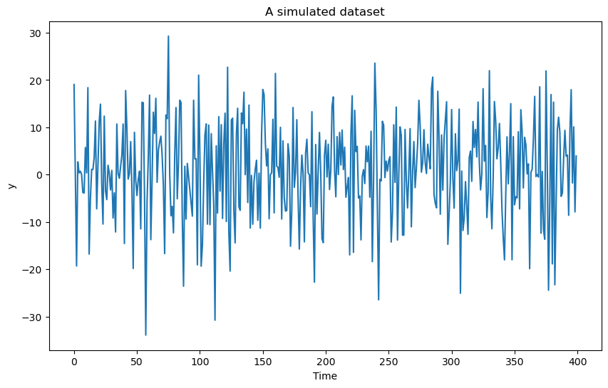

The frequentist solution calculates the MLE. For computing the MLE, we first optimize the following criterion function over $f$ to obtain $\hat{f}$ :

\text{crit}(f) := \min_{\beta_0, \beta_1, \beta_2} \sum_{t=1}^n (y_t - \beta_0 - \beta_1 \cos(2 \pi f t) - \beta_2 \sin(2 \pi f t))^2 = RSS(f),

where $RSS(f)$ denotes the Residual Sum of Squares in the linear regression model obtaining by fixing $f$ . After finding $\hat{f}$ , the MLEs for the other parameters are obtained as in standard linear regression with $f$ fixed at $\hat{f}$ .

def crit(f):
    x = np.arange(1, n + 1)
    xcos = np.cos(2 * np.pi * f * x)
    xsin = np.sin(2 * np.pi * f * x)
    X = np.column_stack([np.ones(n), xcos, xsin])

    md = sm.OLS(y, X).fit()
    rss = np.sum(md.resid ** 2)

    return rss

Here is a plot of $\text{crit}(f)$ as a function of $f$ over a grid of values of $f$ .

ngrid = 100000
allfvals = np.linspace(0, 0.5, ngrid)
critvals = np.array([crit(f) for f in allfvals])

plt.plot(allfvals, critvals)
plt.xlabel('Frequency')
plt.ylabel('Sum of Squares')
plt.title('Least Squares Criterion Function')
plt.show()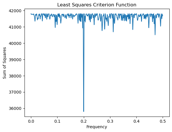

# the MLE of f is now calculated as:
fhat = allfvals[np.argmin(critvals)]

print(fhat)

0.1998969989699897

After obtaining $\hat{f}$ , the estimates of $\beta_0, \beta_1, \beta_2, \sigma$ are obtained in the usual way for linear regression fixing $f = \hat{f}$

x = np.arange(1, n + 1)
xcos = np.cos(2 * np.pi * fhat * x)
xsin = np.sin(2 * np.pi * fhat * x)
Xfhat = np.column_stack([np.ones(n), xcos, xsin])

md = sm.OLS(y, Xfhat).fit()

print(md.params) # this gives estimates of beta_0, beta_1, beta_2
print(md.summary())

[0.98353083 3.62686407 4.11283874]
                            OLS Regression Results                            
==============================================================================
Dep. Variable:                      y   R-squared:                       0.144
Model:                            OLS   Adj. R-squared:                  0.139
Method:                 Least Squares   F-statistic:                     33.33
Date:                Fri, 07 Feb 2025   Prob (F-statistic):           4.16e-14
Time:                        17:35:53   Log-Likelihood:                -1466.4
No. Observations:                 400   AIC:                             2939.
Df Residuals:                     397   BIC:                             2951.
Df Model:                           2                                         
Covariance Type:            nonrobust                                         
==============================================================================
                 coef    std err          t      P>|t|      [0.025      0.975]
------------------------------------------------------------------------------
const          0.9835      0.475      2.071      0.039       0.050       1.917
x1             3.6269      0.672      5.400      0.000       2.307       4.947
x2             4.1128      0.671      6.126      0.000       2.793       5.433
==============================================================================
Omnibus:                        3.795   Durbin-Watson:                   2.183
Prob(Omnibus):                  0.150   Jarque-Bera (JB):                3.854
Skew:                          -0.235   Prob(JB):                        0.146
Kurtosis:                       2.900   Cond. No.                         1.41
==============================================================================

Notes:
[1] Standard Errors assume that the covariance matrix of the errors is correctly specified.

The true values of $\beta_0, \beta_1, \beta_2$ lie in the corresponding 95% C.I given for each coefficient in the model summary above.

# Estimate of sigma:
rss = np.sum(md.resid ** 2)
sigmahat = np.sqrt(rss / (n - 3))

print(sigmahat)

9.495940890783043

Next we look at Bayesian inference which will yield similar results but will additionally provide uncertainty intervals for $f$ . We use the following formula for the Bayesian posterior that we derived in class:

I\{0 \leq f \leq 1/2\} \cdot |X_f^T X_f|^{-1/2} \cdot \left(\frac{1}{S(\hat{\beta}(f), f)} \right)^{(n-p)/2}

where $p = 3$ and $|X_f^T X_f|$ denotes the determinant of $X_f^T X_f$ .

It is better to compute the logarithm of the posterior (as opposed to the posterior directly) because of numerical issues.

def logpost(f):
    x = np.arange(1, n + 1)
    xcos = np.cos(2 * np.pi * f * x)
    xsin = np.sin(2 * np.pi * f * x)
    X = np.column_stack([np.ones(n), xcos, xsin])

    p = X.shape[1]

    md = sm.OLS(y, X).fit()
    rss = np.sum(md.resid ** 2)

    sgn, log_det = np.linalg.slogdet(np.dot(X.T, X)) # sgn gives the sign of the determinant (in our case, this should 1)
    # log_det gives the logarithm of the absolute value of the determinant
    logval = ((p - n) / 2) * np.log(rss) - 0.5 * log_det

    return logval

While evaluating the log posterior on a grid, it is important to make sure that we do not include frequencies $f$ for which $X_f^T X_f$ is singular. This will be the case for $f = 0$ and $f = 1/2$ . When $f$ is very close to 0 or 0.5, the term $|X_f^T X_f|^{-1/2}$ will be very large because of near-singularity of $X_f^T X_f$ . We will therefore exclude frequencies very close to 0 and 0.5 from the grid while calculating posterior probabilities.

logpostvals = np.array([logpost(f) for f in allfvals])

plt.plot(allfvals, logpostvals)
plt.xlabel('Frequency')
plt.ylabel('Value')
plt.title('Logarithm of (unnormalized) posterior density')
plt.show()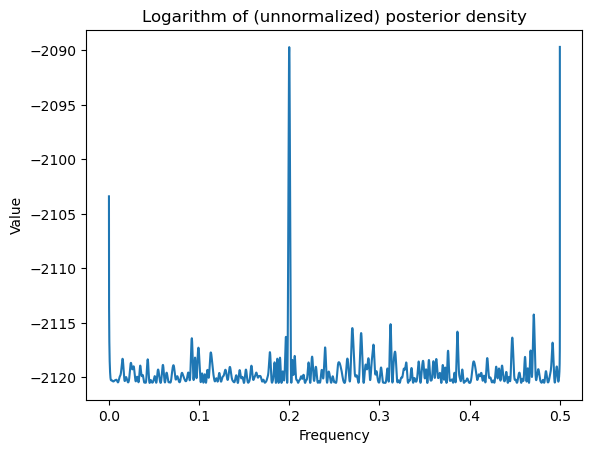

allfvals = allfvals[100:(ngrid - 100)]

print(np.min(allfvals), np.max(allfvals))

logpostvals = np.array([logpost(f) for f in allfvals])

0.0005000050000500005 0.49949999499995

plt.plot(allfvals, logpostvals)
plt.xlabel('Frequency')
plt.ylabel('Value')
plt.title('Logarithm of (unnormalized) posterior density')
plt.show()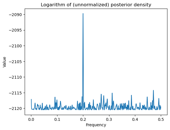

Next we exponentiate the log posterior to obtain posterior. Here we again need to be mindful of numerical issues. If we directly take the exponent of numbers, we might get 0 or ∞. So we first subtract a constant so that the values are somewhat closer to 0 before taking the exponent.

postvals_unnormalized = np.exp(logpostvals - np.max(logpostvals))
postvals = postvals_unnormalized / (np.sum(postvals_unnormalized))

plt.plot(allfvals, postvals)
plt.xlabel('Frequency')
plt.ylabel('Probability')
plt.title('Posterior distribution of frequency')
plt.show()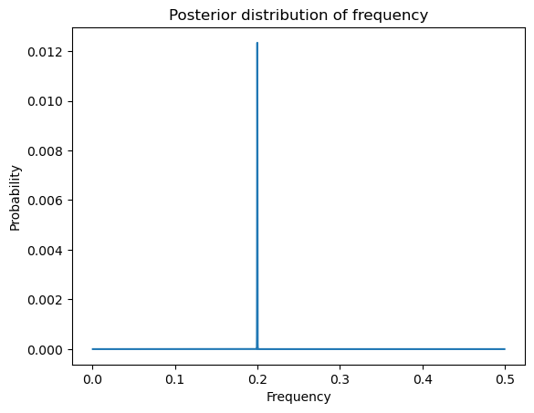

postvals_unnormalized = np.exp(logpostvals - np.max(logpostvals))
postvals_density = postvals_unnormalized / (np.sum(postvals_unnormalized))

postvals_density = postvals_density * (ngrid - 200) / 0.5

plt.plot(allfvals, postvals_density)
plt.xlabel('Frequency')
plt.ylabel('Density')
plt.title('Posterior distribution of frequency')
plt.show()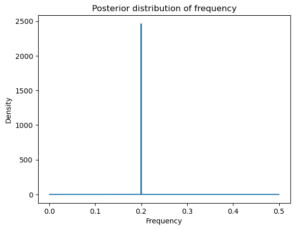

Using the posterior distribution, we can calculate posterior mean etc. and obtain credible intervals for $f$ .

#Posterior mean of f:
fpostmean = np.sum(postvals * allfvals)

#Posterior mode of f:
fpostmode = allfvals[np.argmax(postvals)]

print(fpostmean, fpostmode, fhat)

0.19989514344518863 0.1998969989699897 0.1998969989699897

Note that the posterior mode coincides with the MLE. Let us now compute a credible interval for $f$ . A 95% credible interval is an interval for which the posterior probability is about 95%. The following function takes an input value $m$ and compute the posterior probability assigned to the interval $\hat{f} - m*\delta, \hat{f} + m*\delta$ where δ is the grid resolution that we used for computing the posterior.

def PostProbAroundMax(m):
    est_ind = np.argmax(postvals)
    ans = np.sum(postvals[(est_ind - m):(est_ind + m)])

    return(ans)

We now start with a small value of $m$ (say $m = 0$ ) and keep increasing it until the posterior probability reaches 0.95.

m = 0
while PostProbAroundMax(m) <= 0.95:
    m = m + 1

print(m)

The credible interval for $f$ can then be computed in the following way.

est_ind = np.argmax(postvals)
f_est = allfvals[est_ind]

# 95% credible interval for f:
ci_f_low = allfvals[est_ind - m]
ci_f_high = allfvals[est_ind + m]
print(np.array([f_est, ci_f_low, ci_f_high]))

[0.199897 0.199572 0.200222]

When I implemented this experiment, I found the interval to be very narrow while containing the true value 0.2.

Frequency Aliasing¶

Now consider the same simulation setting as the previous problem but change the true frequency to $f = 1.8$ as opposed to $f = 0.2$ . The analysis then would still yield an estimate which is close to 0.2. This is because the frequency $f_0 = 0.2$ is an alias of $f = 1.8$ in the sense that the two sinusoids $s_t = R \cos (2 \pi f t + \phi)$ and $s_t = R \cos (2 \pi f_0 t - \phi)$ are identical when $t$ is integer-valued. One can note that the estimate of $\beta_2$ will have a flipped sign however.

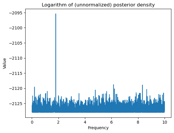
It is very important to note that aliasing is a consequence of our time variable taking the equally spaced values $1, \dots, n$ . If we change the time variable to some non-uniform values (i.e., if we sample the sinusoid at a non-uniform set of values), then it is possible to estimate frequencies which are outside of the range $[0, 0.5]$ . This is illustrated below with $f = 1.8$ . We take time to be randomly chosen points in the range $[1, n]$ .

#f = 0.2
f = 1.8
n = 400
b0 = 0
b1 = 3
b2 = 5
sig = 10

rng = np.random.default_rng()
errorsamples = rng.normal(loc = 0, scale = sig, size = n)

#t = np.arange(1, n+1)
t = np.sort(rng.uniform(low = 1, high = n, size = n))

y = b0 * np.ones(n) + b1 * np.cos(2 * np.pi * f * t) + b2 * np.sin(2 * np.pi * f * t) + errorsamples

print(t) # time again ranges roughly between 1 and 400 but this time the values are not equally spaced

[  1.56329304   2.62935633   3.79388205   3.88731761   3.96842364
   8.54831538  12.83284043  12.95440184  13.09019748  13.23596509
  13.79555142  15.78970998  16.20560962  16.55845882  17.62854352
  17.70651795  19.54620116  19.83031628  20.54486984  23.18637895
  23.38671572  23.81397752  24.9898303   25.74143453  25.75881811
  29.18087541  29.59926001  30.4469271   30.64392491  32.78771125
  33.39879012  35.79954741  36.01481776  38.23331734  39.61847301
  39.62225731  43.95909818  44.17443166  44.56023612  45.17267168
  45.43366364  45.6042612   45.83746185  46.45099859  47.43092162
  47.67447237  48.14188937  48.72066985  51.96628887  52.26213298
  52.9664796   53.79341652  56.9370232   58.68036218  60.94536298
  61.05123473  61.30366849  61.36256233  61.44770438  61.48514674
  62.47577464  62.75035     63.96443712  64.19456149  64.68668648
  67.27881048  67.57517322  67.96705953  70.36120275  70.79681197
  71.59398342  71.96867177  73.49774859  74.32638787  74.7989255
  75.22720993  77.06278269  77.22460502  78.91329867  79.95789269
  80.87339097  83.1697618   85.72464961  86.41130262  86.4606171
  86.91482742  86.97972721  87.12251518  88.64149984  88.98795442
  89.0347649   90.0776779   92.53413579  95.40175094  95.92567657
  98.11842389  98.469774    99.51309954  99.96241524 100.93956851
 101.7963185  101.80730731 103.41862721 103.57346822 103.87394967
 103.96308085 104.24888214 107.28761206 108.68280307 108.79217686
 109.80288815 110.31610772 111.23412454 112.08292937 112.997114
 117.74945423 118.58782992 122.1874555  122.95373767 122.98684483
 124.01625419 125.92102465 132.08080588 133.77996896 134.30060007
 135.39899223 135.93138283 136.37829853 136.95912454 138.03972319
 138.2699533  140.12185619 142.50610008 143.04194124 143.05702832
 145.45142168 146.31585146 148.08548456 149.21460382 152.84780224
 154.20979492 154.27466386 155.77722126 158.60878769 158.79891072
 159.62100619 160.60454449 161.11558922 161.22801599 161.78507292
 162.97014334 164.53799216 165.60232859 166.5335484  167.00985013
 167.55807662 168.62403459 169.9165873  172.03280812 172.97901797
 173.36708297 173.50653259 173.62106753 174.22034325 177.13274235
 177.89009545 178.21670982 179.70669447 180.04482147 181.47039402
 182.25155496 183.3941826  183.8363087  184.45210736 186.36507581
 187.28860965 189.13906978 189.22150662 190.69597724 190.98909976
 191.06452123 191.58906894 192.16455079 192.36164413 194.20480202
 195.41610655 195.84051375 196.43225163 196.72811898 198.30998668
 198.36826137 198.4488313  198.53552647 198.81567354 200.02012444
 201.56072471 202.23470053 202.24262933 203.22455316 203.59994915
 204.48230352 205.41823303 206.37622026 207.40329218 207.87253891
 207.88669486 207.92891413 208.26269795 210.27003942 210.76398451
 211.5801918  213.53839035 216.18385748 219.52282375 220.69941893
 221.72444741 223.43712057 224.51800395 225.63669961 228.01079561
 228.95884607 229.49709447 232.67123976 233.54981155 233.73380512
 234.09345894 234.33478227 234.59001989 236.75936768 238.4499311
 238.68613961 239.16680955 239.5802613  239.77281395 240.16904595
 240.62762214 242.50838113 242.73663604 243.18683195 244.56568321
 247.4385385  248.44449722 249.38740284 250.0406679  250.92616722
 252.08423958 252.15940751 252.57053993 252.8104476  255.29301873
 255.85070122 257.91454977 258.58772416 258.75014578 261.97868346
 263.25229243 263.34714527 263.92527778 264.0364148  265.47553828
 265.80961915 265.88926148 266.58356053 267.68013064 271.80380999
 273.54401589 273.57835952 275.47583185 277.29034781 278.45743694
 279.04555365 279.30996176 280.39253184 280.58770776 281.23605975
 282.36584716 282.57789983 282.70313644 283.52888213 283.54761644
 283.76378146 283.97159456 284.11137391 284.19654782 288.76504076
 289.95635291 290.06760772 292.38058226 292.40356909 293.52821135
 293.68668925 294.40582657 294.46929803 294.70658035 296.01015184
 296.70428527 296.82207851 298.15113412 299.81422665 300.45297084
 301.24877345 301.82638873 302.60557666 303.02937297 303.92319573
 306.47305279 308.31773934 309.29009541 309.44959483 311.16564236
 311.51533257 311.59970593 311.69406182 312.98271272 314.11743519
 314.89667875 315.79190204 317.74680885 318.09126729 318.54572956
 320.06304535 320.12317348 320.36940013 320.75864947 321.06423769
 321.46951554 321.65192651 321.73582711 324.02782528 325.51259126
 327.06025749 328.80504062 329.25958626 329.5863112  329.7164469
 330.29334624 330.57753979 330.5956205  337.17646861 341.70190985
 342.19635652 343.47013609 343.72574087 345.39682723 345.44738567
 347.07987881 349.3707411  349.67101015 350.26048982 351.5933344
 351.807582   353.60896942 355.1997232  356.12874904 360.15593727
 361.01274471 362.00338977 362.90043356 364.03377607 364.66103051
 364.92864053 365.29599151 365.95225971 367.42961622 368.91557754
 369.53157323 370.55137663 371.39653349 372.4944446  372.77157707
 373.42510655 373.43287537 374.27907405 376.50101746 379.12670209
 379.31100572 380.63969551 381.01108968 381.52460312 381.93173212
 382.56276771 383.03506603 383.33386249 383.98859286 384.7596035
 384.87194563 384.89080206 385.87246217 386.15419915 392.28152631
 392.84818043 394.52822668 394.70560108 394.92533504 396.17962428
 397.35689719 399.04555697 399.12513465 399.37177477 399.50260625]

plt.figure(figsize = (10, 6))
plt.plot(y)
plt.xlabel('Time')
plt.ylabel('y')
plt.title('A simulated dataset')
plt.show()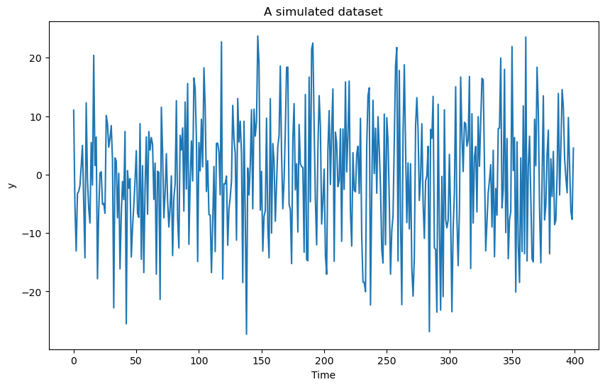

def crit(f):
    xcos = np.cos(2 * np.pi * f * t)
    xsin = np.sin(2 * np.pi * f * t)
    X = np.column_stack([np.ones(n), xcos, xsin])

    md = sm.OLS(y, X).fit()
    rss = np.sum(md.resid ** 2)

    return rss

To evaluate the criterion function, we shall take the grid to be spaced over the larger range $[0, 10]$ . Note that we cannot restrict the frequency parameter to $[0, 1/2]$ because time is not equally spaced.

ngrid = 100000
allfvals = np.linspace(0, 10, ngrid)
critvals = np.array([crit(f) for f in allfvals])

plt.plot(allfvals, critvals)
plt.xlabel('Frequency')
plt.ylabel('Sum of Squares')
plt.title('Least Squares Criterion Function')
plt.show()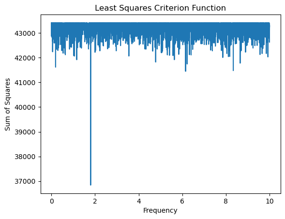

# the MLE of f is now:
fhat = allfvals[np.argmin(critvals)]

print(fhat)

1.7996179961799619

Note that the MLE is very close to 1.8. The Bayesian analysis will also give a posterior that is tightly concentrated around 1.8.

def logpost(f):
    xcos = np.cos(2 * np.pi * f * t)
    xsin = np.sin(2 * np.pi * f * t)
    X = np.column_stack([np.ones(n), xcos, xsin])

    p = X.shape[1]

    md = sm.OLS(y, X).fit()
    rss = np.sum(md.resid ** 2)

    sgn, log_det = np.linalg.slogdet(np.dot(X.T, X)) # sgn gives the sign of the determinant (in our case, this should 1)
    # log_det gives the logarithm of the absolute value of the determinant
    logval = ((p - n) / 2) * np.log(rss) - 0.5 * log_det

    return logval

allfvals = allfvals[100:ngrid] # we are removing some values near 0 to prevent singularity of X_f^T X_f
print(np.min(allfvals), np.max(allfvals))

logpostvals = np.array([logpost(f) for f in allfvals])

plt.plot(allfvals, logpostvals)
plt.xlabel('Frequency')
plt.ylabel('Value')
plt.title('Logarithm of (unnormalized) posterior density')
plt.show()

0.01000010000100001 10.0

postvals_unnormalized = np.exp(logpostvals - np.max(logpostvals))
postvals = postvals_unnormalized / (np.sum(postvals_unnormalized))

plt.plot(allfvals, postvals)
plt.xlabel('Frequency')
plt.ylabel('Probability')
plt.title('Posterior distribution of frequency')
plt.show()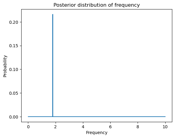

# Posterior mean of f:
fpostmean = np.sum(postvals * allfvals)

# Posterior mode of f:
fpostmode = allfvals[np.argmax(postvals)]

print(fpostmean, fpostmode, fhat)

1.7995875783285253 1.7996179961799619 1.7996179961799619

Stat 153

Sum of Squares and Periodogram