We shall see how simple trend functions can be fit to time series data using linear regression over the time variable (and over other functions of the time variance such as higher powers and sines and cosines). We start with the US population dataset.
US Population Dataset
This dataset is downloaded from FRED and gives monthly population of the United States in thousands.
import pandas as pd
uspop = pd.read_csv('POPTHM-Jan2025FRED.csv')
print(uspop.head(15))
print(uspop.shape)
observation_date POPTHM
0 1959-01-01 175818
1 1959-02-01 176044
2 1959-03-01 176274
3 1959-04-01 176503
4 1959-05-01 176723
5 1959-06-01 176954
6 1959-07-01 177208
7 1959-08-01 177479
8 1959-09-01 177755
9 1959-10-01 178026
10 1959-11-01 178273
11 1959-12-01 178504
12 1960-01-01 178925
13 1960-02-01 179326
14 1960-03-01 179707
(791, 2)
We shall take the covariate variable as which takes the values . Then we shall fit a linear function of to the observed time series using linear regression.
y = uspop['POPTHM']
import numpy as np
x = np.arange(1, len(y)+1) #this is the covariate
import statsmodels.api as sm
X = sm.add_constant(x)
linmod = sm.OLS(y, X).fit()
print(linmod.summary())
print(linmod.params)
OLS Regression Results
==============================================================================
Dep. Variable: POPTHM R-squared: 0.997
Model: OLS Adj. R-squared: 0.997
Method: Least Squares F-statistic: 2.422e+05
Date: Tue, 28 Jan 2025 Prob (F-statistic): 0.00
Time: 19:52:45 Log-Likelihood: -7394.9
No. Observations: 791 AIC: 1.479e+04
Df Residuals: 789 BIC: 1.480e+04
Df Model: 1
Covariance Type: nonrobust
==============================================================================
coef std err t P>|t| [0.025 0.975]
------------------------------------------------------------------------------
const 1.746e+05 198.060 881.427 0.000 1.74e+05 1.75e+05
x1 213.2353 0.433 492.142 0.000 212.385 214.086
==============================================================================
Omnibus: 409.683 Durbin-Watson: 0.000
Prob(Omnibus): 0.000 Jarque-Bera (JB): 73.601
Skew: -0.479 Prob(JB): 1.04e-16
Kurtosis: 1.853 Cond. No. 915.
==============================================================================
Notes:
[1] Standard Errors assume that the covariance matrix of the errors is correctly specified.
const 174575.148609
x1 213.235255
dtype: float64
The estimated slope parameter is 213.2353. The interpretation of this is: the population grows by 213235.255 (note that unit of y is thousands) for every month. The estimated slope parameter is is 174575.148.This is an estimate of the population at time 0 which corresponds to December 1958. The standard errors provide estimates of the uncertainty in and .
To see how well the regression line fits the data, we can plot the line over the original data, as follows.
import matplotlib.pyplot as plt
plt.plot(y, label = "Observed Data")
plt.plot(linmod.fittedvalues, label = 'Fitted Values', color = 'red')
plt.xlabel('Time (months)')
plt.ylabel('Thousands')
plt.title('Population of the United States')
plt.legend()
plt.show()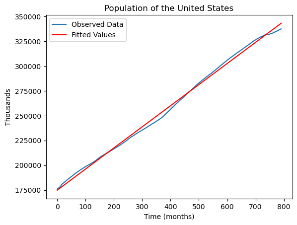
The fit is decent and the line gives a good idea of the overall population growth. However there are some time periods where the population growth diverges from the overall regression line.
The fitted regression line allows us to predict the US population at future time points. This is illustrated below. First note that the given dataset gives population numbers until November 2024:
print(uspop.tail(15)) observation_date POPTHM
776 2023-09-01 335612
777 2023-10-01 335773
778 2023-11-01 335925
779 2023-12-01 336070
780 2024-01-01 336194
781 2024-02-01 336306
782 2024-03-01 336423
783 2024-04-01 336550
784 2024-05-01 336687
785 2024-06-01 336839
786 2024-07-01 337005
787 2024-08-01 337185
788 2024-09-01 337362
789 2024-10-01 337521
790 2024-11-01 337669
The last (791th) observation corresponds to November 2024. Suppose we want to predict the population for January 2025. This corresponds to . The prediction is given by: .
predJan2025 = linmod.params.iloc[0] + 793*linmod.params.iloc[1]
print(predJan2025)
343670.70611584
The predicted US population for January 2025 is therefore 343670.7 million (note the units of are thousands).
linmod supports a function which gives the prediction automatically and also gives uncertainty quantification for the prediction.
print(linmod.get_prediction([1, 793]).summary_frame())
#use linmod.get_prediction([[1, 793], [1, 795]]).summary_frame() to get multiple predictions at x = 793 and x = 795
            mean     mean_se  mean_ci_lower  mean_ci_upper  obs_ci_lower  \
0  343670.706116  198.435157  343281.182823  344060.229409  338194.76474

    obs_ci_upper
0  349146.647492
The get_prediction function gives two uncertainty intervals. The first is for the mean of the prediction, and the second is for the prediction itself. We shall see how these predictions are obtained later. The commonly used uncertainty interval is the second one, which in this case, is .
Google Trends Dataset for the query Amazon
https://
amazon = pd.read_csv('AmazonTrends27Jan2025.csv', skiprows = 1)
#we are skipping the first row as it does not contain any data
print(amazon.head())
amazon.columns = ['Month', 'AmazonTrends']
print(amazon.tail(10))
Month amazon: (United States)
0 2004-01 10
1 2004-02 9
2 2004-03 9
3 2004-04 9
4 2004-05 9
Month AmazonTrends
243 2024-04 61
244 2024-05 66
245 2024-06 65
246 2024-07 68
247 2024-08 63
248 2024-09 60
249 2024-10 60
250 2024-11 63
251 2024-12 72
252 2025-01 61
#Here is a plot of the data
plt.plot(amazon['AmazonTrends'])
plt.xlabel('Time (months)')
plt.ylabel('Search popularity')
plt.title('Google Trends for the query "Amazon"')
plt.show()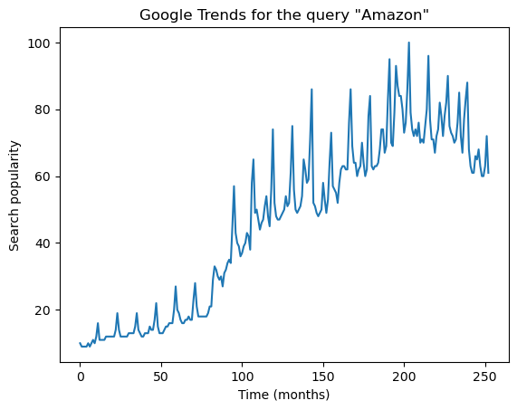
#Fitting a line:
y = amazon['AmazonTrends'] #should we be taking logs instead as in y = np.log(amazon['AmazonTrends'])
x = np.arange(1, len(y) + 1)
X = sm.add_constant(x)
linmod = sm.OLS(y, X).fit()
print(linmod.summary())
OLS Regression Results
==============================================================================
Dep. Variable: AmazonTrends R-squared: 0.856
Model: OLS Adj. R-squared: 0.855
Method: Least Squares F-statistic: 1488.
Date: Tue, 28 Jan 2025 Prob (F-statistic): 1.67e-107
Time: 21:01:31 Log-Likelihood: -933.40
No. Observations: 253 AIC: 1871.
Df Residuals: 251 BIC: 1878.
Df Model: 1
Covariance Type: nonrobust
==============================================================================
coef std err t P>|t| [0.025 0.975]
------------------------------------------------------------------------------
const 5.4659 1.226 4.458 0.000 3.051 7.881
x1 0.3229 0.008 38.581 0.000 0.306 0.339
==============================================================================
Omnibus: 18.674 Durbin-Watson: 0.509
Prob(Omnibus): 0.000 Jarque-Bera (JB): 34.128
Skew: 0.405 Prob(JB): 3.88e-08
Kurtosis: 4.607 Cond. No. 294.
==============================================================================
Notes:
[1] Standard Errors assume that the covariance matrix of the errors is correctly specified.
plt.plot(y, label = 'Original Data')
plt.plot(linmod.fittedvalues, label = "Fitted values")
plt.xlabel('Time (months)')
plt.ylabel('Search popularity')
plt.title('Google search popularity for "Amazon"')
plt.legend()
plt.show()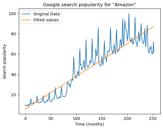
The line does not capture the trend in the data well. We can improve the model by adding a quadratic term.
#Let us add a quadratic term:
x2 = x ** 2
X = np.column_stack([x, x2])
X = sm.add_constant(X)
quadmod = sm.OLS(y, X).fit()
print(quadmod.summary())
OLS Regression Results
==============================================================================
Dep. Variable: AmazonTrends R-squared: 0.877
Model: OLS Adj. R-squared: 0.876
Method: Least Squares F-statistic: 889.5
Date: Tue, 28 Jan 2025 Prob (F-statistic): 2.14e-114
Time: 21:01:33 Log-Likelihood: -913.42
No. Observations: 253 AIC: 1833.
Df Residuals: 250 BIC: 1843.
Df Model: 2
Covariance Type: nonrobust
==============================================================================
coef std err t P>|t| [0.025 0.975]
------------------------------------------------------------------------------
const -2.9098 1.711 -1.700 0.090 -6.280 0.461
x1 0.5199 0.031 16.713 0.000 0.459 0.581
x2 -0.0008 0.000 -6.541 0.000 -0.001 -0.001
==============================================================================
Omnibus: 21.416 Durbin-Watson: 0.596
Prob(Omnibus): 0.000 Jarque-Bera (JB): 25.310
Skew: 0.660 Prob(JB): 3.19e-06
Kurtosis: 3.812 Cond. No. 8.70e+04
==============================================================================
Notes:
[1] Standard Errors assume that the covariance matrix of the errors is correctly specified.
[2] The condition number is large, 8.7e+04. This might indicate that there are
strong multicollinearity or other numerical problems.
plt.plot(y, label = 'Original Data', color = 'blue')
plt.plot(linmod.fittedvalues, label = "Fitted (linear)", color = 'red')
plt.plot(quadmod.fittedvalues, label = "Fitted (quadratic)", color = 'black')
plt.xlabel('Time (months)')
plt.ylabel('Search popularity')
plt.title('Google search popularity for "Amazon"')
plt.legend()
plt.show()
The fit is still not good. Let us add a cubic term.
#Cubic term:
x2 = x ** 2
x3 = x ** 3
X = np.column_stack([x, x2, x3])
X = sm.add_constant(X)
cubmod = sm.OLS(y, X).fit()
print(cubmod.summary())
OLS Regression Results
==============================================================================
Dep. Variable: AmazonTrends R-squared: 0.921
Model: OLS Adj. R-squared: 0.920
Method: Least Squares F-statistic: 965.6
Date: Tue, 28 Jan 2025 Prob (F-statistic): 8.78e-137
Time: 21:01:36 Log-Likelihood: -857.44
No. Observations: 253 AIC: 1723.
Df Residuals: 249 BIC: 1737.
Df Model: 3
Covariance Type: nonrobust
==============================================================================
coef std err t P>|t| [0.025 0.975]
------------------------------------------------------------------------------
const 11.5863 1.845 6.279 0.000 7.952 15.221
x1 -0.1582 0.063 -2.520 0.012 -0.282 -0.035
x2 0.0059 0.001 10.257 0.000 0.005 0.007
x3 -1.749e-05 1.49e-06 -11.773 0.000 -2.04e-05 -1.46e-05
==============================================================================
Omnibus: 62.554 Durbin-Watson: 0.926
Prob(Omnibus): 0.000 Jarque-Bera (JB): 123.235
Skew: 1.247 Prob(JB): 1.74e-27
Kurtosis: 5.338 Cond. No. 2.50e+07
==============================================================================
Notes:
[1] Standard Errors assume that the covariance matrix of the errors is correctly specified.
[2] The condition number is large, 2.5e+07. This might indicate that there are
strong multicollinearity or other numerical problems.
plt.figure(figsize = (10, 6))
plt.plot(y, label = 'Original Data', color = 'blue')
plt.plot(linmod.fittedvalues, label = "Fitted (linear)", color = 'red')
plt.plot(quadmod.fittedvalues, label = "Fitted (quadratic)", color = 'black')
plt.plot(cubmod.fittedvalues, label = "Fitted (cubic)", color = 'green')
plt.xlabel('Time (months)')
plt.ylabel('Search popularity')
plt.title('Google search popularity for "Amazon"')
plt.legend()
plt.show()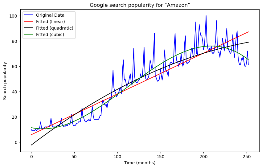
Now the fit is pretty good. This is a monthly dataset which also has a clear seasonal pattern. Some months in each year have a high value compared to other months. We can capture this seasonal pattern by adding cosines and sines to the regression model. The simplest seasonal functions with period 12 are and . Let us add these to the model.
#Adding seasonal terms to the model:
x4 = np.cos(2 * np.pi * x * (1/12))
x5 = np.sin(2 * np.pi * x * (1/12))
X = np.column_stack([x, x2, x3, x4, x5])
X = sm.add_constant(X)
seasmod1 = sm.OLS(y, X).fit()
plt.figure(figsize = (10, 6))
plt.plot(y, label = 'Original Data', color = 'blue')
plt.plot(cubmod.fittedvalues, label = "Fitted (cubic)", color = 'red')
plt.plot(seasmod1.fittedvalues, label = "Fitted (with seasonal term)", color = 'black')
plt.xlabel('Time (months)')
plt.ylabel('Search popularity')
plt.title('Google search popularity for "Amazon"')
plt.legend()
plt.show()
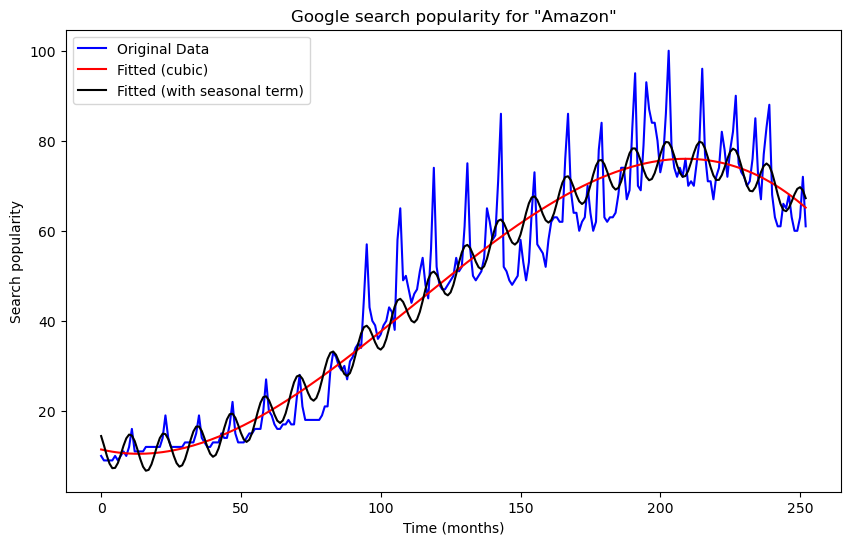
The fit is better but the seasonal term is not enough to capture the actual oscillation present in the data. We improve the fit by adding two more seasonal functions and .
#Adding seasonal terms to the model:
x4 = np.cos(2 * np.pi * x * (1/12))
x5 = np.sin(2 * np.pi * x * (1/12))
x6 = np.cos(2 * np.pi * x * (2/12))
x7 = np.sin(2 * np.pi * x * (2/12))
X = np.column_stack([x, x2, x3, x4, x5, x6, x7])
X = sm.add_constant(X)
seasmod = sm.OLS(y, X).fit()
plt.figure(figsize = (10, 6))
plt.plot(y, label = 'Original Data', color = 'blue')
plt.plot(cubmod.fittedvalues, label = "Fitted (cubic)", color = 'red')
plt.plot(seasmod.fittedvalues, label = "Fitted (with seasonal term)", color = 'black')
plt.xlabel('Time (months)')
plt.ylabel('Search popularity')
plt.title('Google search popularity for "Amazon"')
plt.legend()
plt.show()
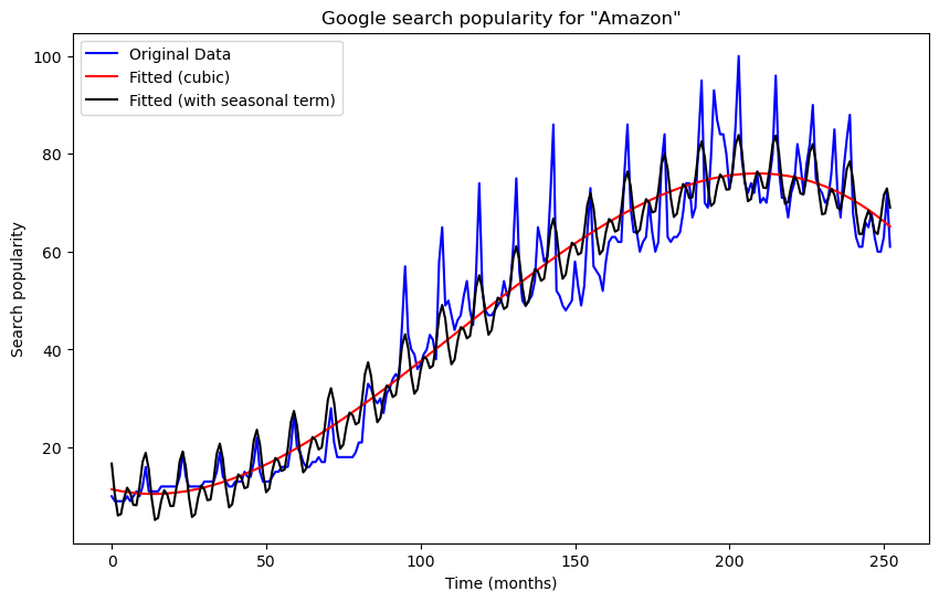
The fit is much improved (even though there is still some discrepancy between the seasonal oscillations in the data and the fitted function). We can use this model to predict the data for a bunch of future time points.
#Computing future predictions:
nf = 100 #number of future points where we are calculating predictions
xf = np.arange(len(x) + 1, len(x) + 1 + nf) #these are the future time points
x2f = xf ** 2
x3f = xf ** 3
x4f = np.cos(2 * np.pi * xf * (1/12))
x5f = np.sin(2 * np.pi * xf * (1/12))
x6f = np.cos(2 * np.pi * xf * (2/12))
x7f = np.sin(2 * np.pi * xf * (2/12))
Xf = np.column_stack([xf, x2f, x3f, x4f, x5f, x6f, x7f])
Xf = sm.add_constant(Xf)
pred = Xf @ np.array(seasmod.params) #these are the predictions
print(pred)
[ 62.33354419 57.5707147 57.4025666 60.14123908 61.78180958
60.18068867 57.16397471 56.46682572 59.62728959 64.04014559
65.2262396 61.13794896 54.24182287 49.28634604 48.92424875
51.4676702 52.91168785 51.11271224 47.89684175 46.9992344
49.95793806 54.16773202 55.14946216 50.8555058 43.75241217
38.58866595 38.01699745 40.34954585 41.5813886 39.56893627
36.13828721 35.02459946 37.76592089 41.75703078 42.51877502
38.00353092 30.67784771 25.29021008 24.49334832 26.59940163
27.60344746 25.36189637 21.70084672 20.35545654 22.86377371
26.62057749 27.14671379 22.39455992 14.83066509 9.20351402
8.16583698 10.02977318 10.79040005 8.30412817 4.39705589
2.80434125 5.06403212 8.57090777 8.84581409 3.84112841
-3.97660005 -9.85888661 -11.15300096 -9.54680391 -9.04521802
-11.79183273 -15.96054966 -17.8162108 -15.82076826 -12.57944278
-12.57138845 -17.84422797 -25.93141211 -32.08445618 -33.65062987
-32.31779401 -32.09087114 -35.1134507 -39.55943432 -41.69366398
-39.97809181 -37.01793852 -37.29235823 -42.84897362 -51.22123547
-57.66065908 -59.51451415 -58.4706615 -58.53402368 -61.84819013
-66.58706247 -69.01548269 -67.59540292 -64.93204386 -65.50455963
-71.36057292 -80.03353451 -86.77495969 -88.93211818 -88.19287077]
#Plotting the data, fitted values and predictions
xall = np.concatenate([x, xf])
fittedpred = np.concatenate([seasmod.fittedvalues, pred])
#plt.figure(figsize = (10, 6))
#print(x)
#print(xf)
plt.plot(xall, fittedpred, color = 'gray', label = 'Fitted values')
plt.plot(xf, pred, color = 'red', label = 'Predictions')
plt.plot(x, y, label = 'Original Data', color = 'blue')
plt.legend()
plt.show()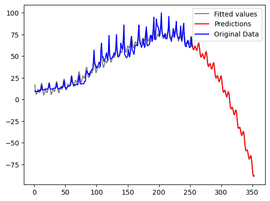
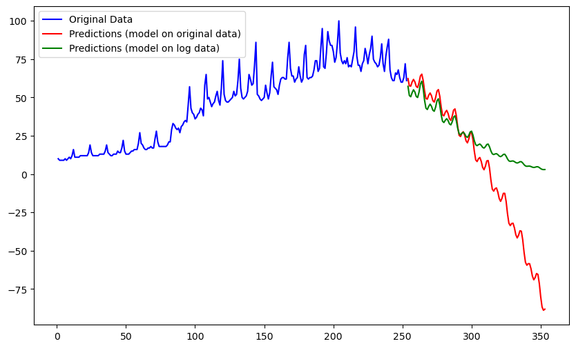
Note that the future predictions become negative after a certain time. This is because the predictions follow the decreasing trend in the cubic function near the right end of the dataset. In this particular problem, negative predictions are meaningless. This issue can be fixed if we fit models to the logarithms of the original data. The model predictions will then have to be exponentiated if we want predictions for the original data. This exponentiation will ensure that all predictions are positive.
#Prediction on log(data):
ylog = np.log(amazon['AmazonTrends'])
seasmodlog = sm.OLS(ylog, X).fit()
predlog = Xf @ np.array(seasmodlog.params)
print(predlog)

xall = np.concatenate([x, xf])
fittedpred_logmodel = np.concatenate([np.exp(seasmodlog.fittedvalues), np.exp(predlog)])
plt.figure(figsize = (10, 6))
#print(x)
#print(xf)
plt.plot(x, y, label = 'Original Data', color = 'blue')
plt.plot(xf, pred, color = 'red', label = 'Predictions (model on original data)')
#plt.plot(xall, fittedpred_logmodel, color = 'black')
plt.plot(xf, np.exp(predlog), color = 'green',  label = 'Predictions (model on log data)')
plt.legend()
plt.show()
[4.04755544 3.93709815 3.92125227 3.97179077 4.00777692 3.98106626
3.92404976 3.91200234 3.97909707 4.07440479 4.10451207 4.02236631
3.87472641 3.76066131 3.74118872 3.7880816 3.82040325 3.79000916
3.72929035 3.7135217 3.77687631 3.868425 3.89475435 3.80881176
3.65735612 3.53945639 3.51613026 3.55915071 3.58758101 3.55327668
3.48862872 3.46891202 3.52829968 3.61586252 3.63818711 3.54822086
3.39272267 3.27076148 3.24335498 3.28227616 3.30658829 3.26814689
3.19934296 3.17545139 3.23064527 3.31399543 3.33208844 3.23787171
3.07810413 2.95185464 2.92014096 2.95473604 2.97470318 2.93189788
2.85871115 2.83041787 2.88119115 2.9601018 2.9737364 2.87504236
2.71077857 2.58001397 2.54376626 2.57380843 2.58920374 2.54180772
2.46401136 2.43108956 2.4772154 2.55145972 2.56040909 2.45701091
2.28802407 2.15251753 2.11150898 2.1367714 2.14736807 2.09515449
2.01252168 1.97474452 2.01599611 2.08534727 2.08938457 1.98105542
1.80711872 1.66664341 1.62064719 1.64090304 1.64647423 1.58921628
1.50152018 1.45866084 1.49481134 1.55904251 1.55794093 1.44445399
1.2653406 1.11966969 1.06845897 1.08348142]