import numpy as np
import pandas as pd
import matplotlib.pyplot as plt
import statsmodels.api as sm
We will fit AutoRegressive Models to some time series datasets, and obtain predictions for future values of the time series.
Dataset One: Liquor Sales Data from FRED
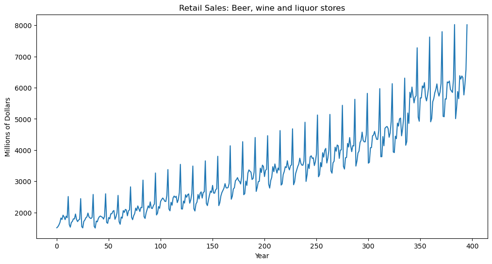
#The following is FRED data on retail sales (in millions of dollars) for beer, wine and liquor stores (https://fred.stlouisfed.org/series/MRTSSM4453USN)
beersales = pd.read_csv('MRTSSM4453USN_March2025.csv')
print(beersales.head())
y = beersales['MRTSSM4453USN'].to_numpy()
plt.figure(figsize = (12, 6))
plt.plot(y)
plt.xlabel('Year')
plt.ylabel('Millions of Dollars')
plt.title('Retail Sales: Beer, wine and liquor stores')
plt.show()
observation_date MRTSSM4453USN
0 1992-01-01 1509
1 1992-02-01 1541
2 1992-03-01 1597
3 1992-04-01 1675
4 1992-05-01 1822
AutoRegressive (AR) models are a simple way for obtaining forecasts (predictions) for future values of the time series.
p = 12 #this is the order of the AR model
n = len(y)
print(n)
print(y)
396
[1509 1541 1597 1675 1822 1775 1912 1862 1770 1882 1831 2511 1614 1529
1678 1713 1796 1792 1950 1777 1707 1757 1782 2443 1548 1505 1714 1757
1830 1857 1981 1858 1823 1806 1845 2577 1555 1501 1725 1699 1807 1863
1886 1861 1845 1788 1879 2598 1679 1652 1837 1798 1957 1958 2034 2062
1781 1860 1992 2547 1706 1621 1853 1817 2060 2002 2098 2079 1892 2050
2082 2821 1846 1768 1894 1963 2140 2059 2209 2118 2031 2163 2154 3037
1866 1808 1986 2099 2210 2145 2339 2140 2126 2219 2273 3265 1920 1976
2190 2132 2357 2413 2463 2422 2358 2352 2549 3375 2109 2052 2327 2231
2470 2526 2483 2518 2316 2409 2638 3542 2114 2109 2366 2300 2569 2486
2568 2595 2297 2401 2601 3488 2121 2046 2273 2333 2576 2433 2611 2660
2461 2641 2660 3654 2293 2219 2398 2553 2685 2643 2867 2622 2618 2727
2763 3801 2219 2316 2530 2640 2709 2783 2924 2791 2784 2801 2933 4137
2424 2519 2753 2791 3017 3055 3117 3024 2997 2913 3137 4269 2569 2603
3005 2867 3262 3364 3322 3292 3057 3087 3297 4403 2675 2806 2989 2997
3420 3279 3517 3472 3151 3351 3386 4461 2913 2781 3024 3130 3467 3307
3555 3399 3263 3425 3356 4625 2878 2916 3214 3310 3467 3438 3657 3454
3365 3497 3524 4681 2888 2984 3249 3363 3471 3551 3740 3576 3517 3515
3646 4892 2995 3202 3550 3409 3786 3816 3733 3752 3503 3626 3869 5124
3143 3211 3601 3463 3915 3773 3993 4054 3586 3738 4004 5143 3331 3258
3594 3641 4092 3963 4162 4135 3733 3998 4007 5435 3480 3391 3755 3761
4215 4097 4401 4134 3949 4141 4131 5628 3487 3643 3908 3967 4244 4310
4575 4312 4264 4265 4492 5818 3580 3609 4076 4079 4457 4482 4598 4451
4344 4341 4636 5969 3787 3788 4433 4138 4698 4736 4757 4691 4411 4550
4925 6129 3939 3919 4446 4364 4865 4768 5001 5025 4457 4680 5051 6307
4155 4274 5188 4855 5853 5683 6020 5742 5513 5696 5738 7279 5056 4924
5674 5668 6056 5993 6163 5711 5576 5759 6009 7623 4906 5016 5547 5652
5839 5947 6120 5867 5730 5855 6134 7796 5080 5068 5642 5634 6184 6157
6213 5947 5894 5847 6288 8023 5007 5360 5876 5646 6385 6273 6375 6324
5768 6104 6577 8017]
AR models work just like regression. The response vector and design matrix in the regression are set up as follows.
yreg = y[p:] #these are the response values in the autoregression
Xmat = np.ones((n-p, 1)) #this will be the design matrix (X) in the autoregression
for j in range(1, p+1):
    col = y[p-j : n-j]
    Xmat = np.column_stack([Xmat, col])
print(Xmat.shape)
print(Xmat)
(384, 13)
[[1.000e+00 2.511e+03 1.831e+03 ... 1.597e+03 1.541e+03 1.509e+03]
[1.000e+00 1.614e+03 2.511e+03 ... 1.675e+03 1.597e+03 1.541e+03]
[1.000e+00 1.529e+03 1.614e+03 ... 1.822e+03 1.675e+03 1.597e+03]
...
[1.000e+00 5.768e+03 6.324e+03 ... 8.023e+03 6.288e+03 5.847e+03]
[1.000e+00 6.104e+03 5.768e+03 ... 5.007e+03 8.023e+03 6.288e+03]
[1.000e+00 6.577e+03 6.104e+03 ... 5.360e+03 5.007e+03 8.023e+03]]
armod = sm.OLS(yreg, Xmat).fit()
print(armod.summary())
OLS Regression Results
==============================================================================
Dep. Variable: y R-squared: 0.988
Model: OLS Adj. R-squared: 0.988
Method: Least Squares F-statistic: 2552.
Date: Thu, 13 Mar 2025 Prob (F-statistic): 0.00
Time: 23:45:11 Log-Likelihood: -2478.8
No. Observations: 384 AIC: 4984.
Df Residuals: 371 BIC: 5035.
Df Model: 12
Covariance Type: nonrobust
==============================================================================
coef std err t P>|t| [0.025 0.975]
------------------------------------------------------------------------------
const -15.7845 22.657 -0.697 0.486 -60.336 28.767
x1 0.0294 0.018 1.661 0.098 -0.005 0.064
x2 0.0407 0.018 2.296 0.022 0.006 0.076
x3 0.0511 0.018 2.901 0.004 0.016 0.086
x4 0.0287 0.018 1.621 0.106 -0.006 0.063
x5 0.0487 0.018 2.743 0.006 0.014 0.084
x6 0.0104 0.018 0.580 0.562 -0.025 0.046
x7 -0.0028 0.018 -0.157 0.876 -0.038 0.032
x8 -0.0210 0.018 -1.181 0.238 -0.056 0.014
x9 -0.0382 0.018 -2.149 0.032 -0.073 -0.003
x10 -0.0583 0.018 -3.288 0.001 -0.093 -0.023
x11 -0.0176 0.018 -0.988 0.324 -0.053 0.017
x12 0.9692 0.018 54.000 0.000 0.934 1.005
==============================================================================
Omnibus: 172.409 Durbin-Watson: 0.858
Prob(Omnibus): 0.000 Jarque-Bera (JB): 1166.518
Skew: 1.771 Prob(JB): 4.94e-254
Kurtosis: 10.769 Cond. No. 3.59e+04
==============================================================================
Notes:
[1] Standard Errors assume that the covariance matrix of the errors is correctly specified.
[2] The condition number is large, 3.59e+04. This might indicate that there are
strong multicollinearity or other numerical problems.
arfitted = armod.fittedvalues
#Plotting the original data and the fitted values:
plt.plot(figure = (12, 6))
plt.plot(yreg)
plt.plot(arfitted, color = 'red', label = 'Fitted')
plt.show()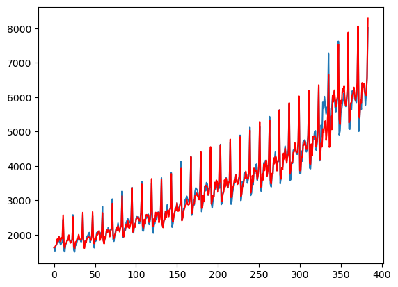
#Generate k-step ahead forecasts:
k = 100
yhat = np.concatenate([y, np.full(k, -9999)]) #extend data by k placeholder values
for i in range(1, k+1):
    ans = armod.params[0]
    for j in range(1, p+1):
        ans += armod.params[j] * yhat[n+i-j-1]
    yhat[n+i-1] = ans
predvalues = yhat[n:]
#Plotting the series with forecasts:
plt.figure(figsize=(12, 6))
time_all = np.arange(1, n + k + 1)
plt.plot(time_all, yhat, label='Extended Series (yhat)', color='C0')
plt.plot(range(1, n + 1), y, label='Original Data', color='C1')
plt.plot(range(n + 1, n + k + 1), predvalues, label='Forecasts', color='blue')
plt.axvline(x=n, color='black', linestyle='--', label='Forecast Start')
#plt.axhline(y=np.mean(y), color='gray', linestyle=':', label='Mean of Original Data')
plt.xlabel('Time')
plt.ylabel('Data')
plt.title('Time Series + AR(p) Forecasts')
plt.legend()
plt.show()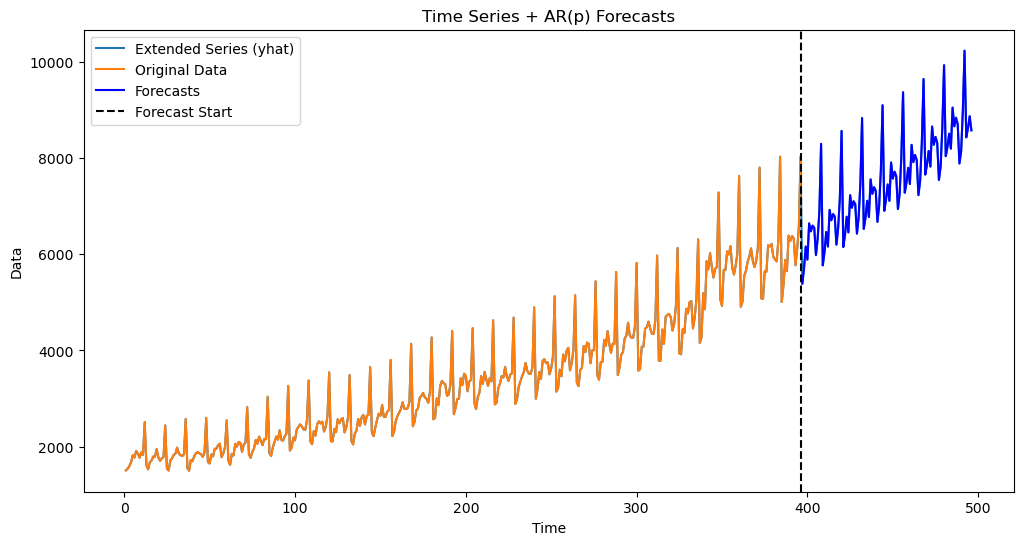
The predictions depend crucially on the order of the model. If , we get reasonable predictions. However for smaller values of , the predictions look very unnatural. Go back and repeat the code above for other values of .
Dataset Two: House Price Data from FRED
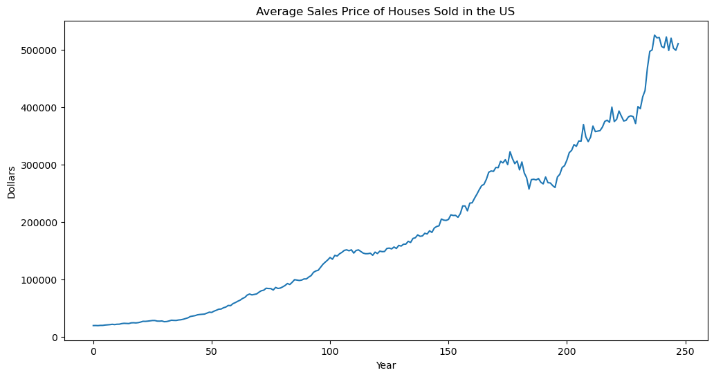
#The following is FRED data on Average Sales Price of Houses Sold for the US (https://fred.stlouisfed.org/series/ASPUS)
hprice = pd.read_csv('ASPUS_March2025.csv')
print(hprice.head())
y = hprice['ASPUS'].to_numpy()
plt.figure(figsize = (12, 6))
plt.plot(y)
plt.xlabel('Year')
plt.ylabel('Dollars')
plt.title('Average Sales Price of Houses Sold in the US')
plt.show()
observation_date ASPUS
0 1963-01-01 19300
1 1963-04-01 19400
2 1963-07-01 19200
3 1963-10-01 19600
4 1964-01-01 19600
p = 30 #this is the order of the AR model
n = len(y)
print(n)
248
yreg = y[p:] #these are the response values in the autoregression
Xmat = np.ones((n-p, 1)) #this will be the design matrix (X) in the autoregression
for j in range(1, p+1):
    col = y[p-j : n-j].reshape(-1, 1)
    Xmat = np.column_stack([Xmat, col])
print(Xmat.shape)
print(y)
(218, 31)
[ 19300 19400 19200 19600 19600 20200 20500 20900 21500 21000
21600 21700 22700 23200 23000 22800 24000 24200 23900 24400
25400 26700 26600 27000 27600 28100 28100 27100 27000 27300
26000 26300 27300 28600 28300 28200 29000 29400 30300 31600
32800 35100 35900 36600 38000 38600 39000 39300 40900 42600
42200 44400 46000 47800 48100 50300 51600 54300 54000 57500
59300 61600 63500 66400 68300 72400 74200 72700 73600 74400
77500 80000 80900 84300 83800 83700 81200 85700 83900 84600
86700 89100 92500 90800 94700 99200 98500 97800 98500 100500
100500 103800 106300 112000 114400 115600 120800 126100 129900 133500
137900 134800 141500 140400 144300 146800 150200 151200 149500 151200
145500 150100 151100 148200 145400 144400 144500 145300 141700 147200
144700 148900 148000 148300 153600 154200 152800 156100 153500 158900
157700 160900 161100 166000 164000 171000 172200 177200 174700 175400
180000 178800 184300 181500 189100 191800 193000 204800 202900 202400
204100 212100 211000 211200 207800 214200 227600 227600 219100 232500
233100 241000 248100 256000 262900 265300 274000 286300 288500 287800
294600 294200 305300 302600 308100 299600 322100 310100 301200 305800
290400 304200 285100 276600 257000 273400 274100 272900 275300 268800
266000 278000 268100 267600 263000 259700 278000 282700 294500 297700
307400 320400 324400 334400 331400 340600 340400 369400 348000 339700
347400 366700 357000 357900 358800 364900 374800 376900 373200 399700
374600 378400 392900 384000 375500 376700 382700 384600 383000 371100
400600 396900 417400 428600 468000 496700 499300 525100 520300 521000
505300 503000 521900 498300 519700 502200 498700 510300]
armod = sm.OLS(yreg, Xmat).fit()
print(armod.summary())
OLS Regression Results
==============================================================================
Dep. Variable: y R-squared: 0.998
Model: OLS Adj. R-squared: 0.997
Method: Least Squares F-statistic: 2805.
Date: Thu, 13 Mar 2025 Prob (F-statistic): 8.59e-232
Time: 16:17:10 Log-Likelihood: -2216.9
No. Observations: 218 AIC: 4496.
Df Residuals: 187 BIC: 4601.
Df Model: 30
Covariance Type: nonrobust
==============================================================================
coef std err t P>|t| [0.025 0.975]
------------------------------------------------------------------------------
const 1362.7186 893.733 1.525 0.129 -400.376 3125.813
x1 0.7860 0.073 10.749 0.000 0.642 0.930
x2 0.5475 0.094 5.848 0.000 0.363 0.732
x3 -0.2009 0.102 -1.968 0.051 -0.402 0.000
x4 -0.0526 0.102 -0.518 0.605 -0.253 0.148
x5 0.0467 0.101 0.463 0.644 -0.152 0.245
x6 -0.3590 0.098 -3.664 0.000 -0.552 -0.166
x7 0.0043 0.101 0.042 0.966 -0.196 0.205
x8 0.1898 0.102 1.859 0.065 -0.012 0.391
x9 0.1898 0.104 1.821 0.070 -0.016 0.395
x10 -0.2491 0.103 -2.417 0.017 -0.452 -0.046
x11 0.0068 0.107 0.064 0.949 -0.204 0.218
x12 0.3036 0.105 2.886 0.004 0.096 0.511
x13 -0.4766 0.110 -4.325 0.000 -0.694 -0.259
x14 -0.1386 0.115 -1.201 0.231 -0.366 0.089
x15 0.6107 0.117 5.208 0.000 0.379 0.842
x16 -0.0564 0.123 -0.458 0.647 -0.299 0.186
x17 -0.2568 0.125 -2.055 0.041 -0.503 -0.010
x18 0.1249 0.120 1.040 0.300 -0.112 0.362
x19 0.1171 0.118 0.992 0.323 -0.116 0.350
x20 -0.1026 0.118 -0.870 0.386 -0.335 0.130
x21 -0.2723 0.119 -2.286 0.023 -0.507 -0.037
x22 0.1050 0.119 0.885 0.377 -0.129 0.339
x23 0.0348 0.119 0.292 0.771 -0.200 0.270
x24 -0.2470 0.118 -2.086 0.038 -0.481 -0.013
x25 0.5378 0.116 4.629 0.000 0.309 0.767
x26 0.0990 0.124 0.796 0.427 -0.146 0.344
x27 -0.5720 0.123 -4.640 0.000 -0.815 -0.329
x28 0.2559 0.130 1.971 0.050 -0.000 0.512
x29 0.1036 0.126 0.821 0.413 -0.145 0.352
x30 -0.0665 0.107 -0.623 0.534 -0.277 0.144
==============================================================================
Omnibus: 31.034 Durbin-Watson: 1.997
Prob(Omnibus): 0.000 Jarque-Bera (JB): 93.321
Skew: 0.553 Prob(JB): 5.44e-21
Kurtosis: 6.008 Cond. No. 2.27e+06
==============================================================================
Notes:
[1] Standard Errors assume that the covariance matrix of the errors is correctly specified.
[2] The condition number is large, 2.27e+06. This might indicate that there are
strong multicollinearity or other numerical problems.
arfitted = armod.fittedvalues
#Plotting the original data and the fitted values:
plt.plot(figure = (12, 6))
plt.plot(yreg)
plt.plot(arfitted, color = 'red', label = 'Fitted')
plt.show()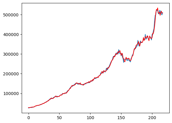
#Generate k-step ahead forecasts:
k = 100
yhat = np.concatenate([y, np.full(k, -9999)]) #extend data by k placeholder values
for i in range(1, k+1):
    ans = armod.params[0]
    for j in range(1, p+1):
        ans += armod.params[j] * yhat[n+i-j-1]
    yhat[n+i-1] = ans
predvalues = yhat[n:]
#Plotting the series with forecasts:
plt.figure(figsize=(12, 6))
time_all = np.arange(1, n + k + 1)
plt.plot(time_all, yhat, label='Extended Series (yhat)', color='C0')
plt.plot(range(1, n + 1), y, label='Original Data', color='C1')
plt.plot(range(n + 1, n + k + 1), predvalues, label='Forecasts', color='blue')
plt.axvline(x=n, color='black', linestyle='--', label='Forecast Start')
#plt.axhline(y=np.mean(y), color='gray', linestyle=':', label='Mean of Original Data')
plt.xlabel('Time')
plt.ylabel('Data')
plt.title('Time Series + AR(p) Forecasts')
plt.legend()
plt.show()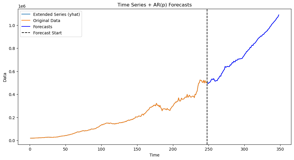
Repeat the above code for different values of to see how the predictions change.
Sunspots Data
We will apply AR models to the sunspots data and obtain predictions.
sunspots = pd.read_csv('SN_y_tot_V2.0.csv', header = None, sep = ';')
y = sunspots.iloc[:,1].values
n = len(y)
plt.figure(figsize = (12, 6))
plt.plot(y)
plt.show()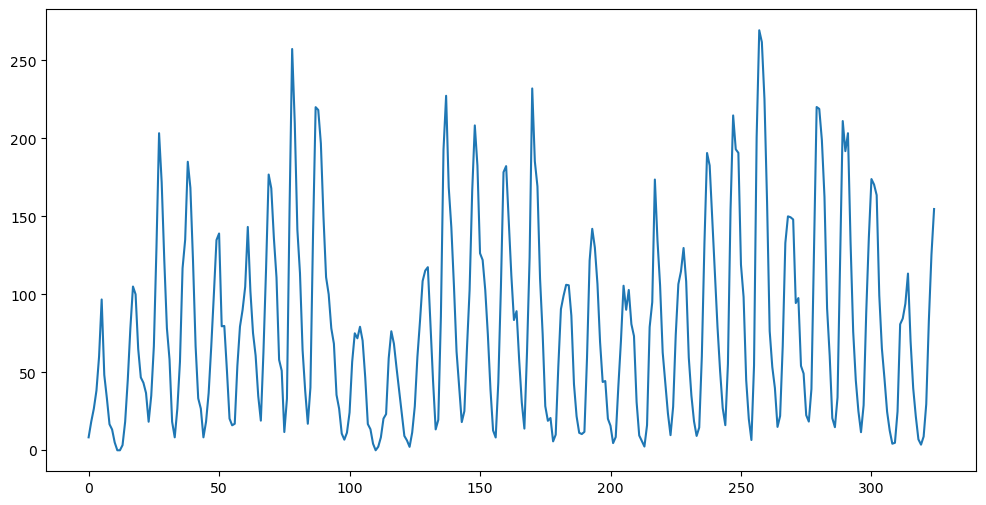
Yule Model
Yule model is given by:
Note that in the usual AR(2) model is set to -1 above. Also is given by . The above model can be rewritten as
so we can estimate and by regressing on .
p = 2
yreg = y[p:]
x1 = y[1:-1]
x2 = y[:-2]
Xmat = np.column_stack([np.ones(len(yreg)), x1])
print(Xmat.shape)(323, 2)
y_adjusted = yreg + x2
yulemod = sm.OLS(y_adjusted, Xmat).fit()
print(yulemod.summary())
print(yulemod.params)
slpe_est = yulemod.params[1] OLS Regression Results
==============================================================================
Dep. Variable: y R-squared: 0.930
Model: OLS Adj. R-squared: 0.930
Method: Least Squares F-statistic: 4254.
Date: Thu, 13 Mar 2025 Prob (F-statistic): 2.90e-187
Time: 23:52:45 Log-Likelihood: -1532.1
No. Observations: 323 AIC: 3068.
Df Residuals: 321 BIC: 3076.
Df Model: 1
Covariance Type: nonrobust
==============================================================================
coef std err t P>|t| [0.025 0.975]
------------------------------------------------------------------------------
const 28.6834 2.511 11.421 0.000 23.742 33.624
x1 1.6365 0.025 65.224 0.000 1.587 1.686
==============================================================================
Omnibus: 11.119 Durbin-Watson: 2.493
Prob(Omnibus): 0.004 Jarque-Bera (JB): 17.202
Skew: 0.225 Prob(JB): 0.000184
Kurtosis: 4.037 Cond. No. 162.
==============================================================================
Notes:
[1] Standard Errors assume that the covariance matrix of the errors is correctly specified.
[28.6833743 1.63648935]
From the estimate for , the frequency parameter can be estimated using the relation: .
yulefhat = np.arccos(slpe_est/2) / (2 * np.pi)
print(1/yulefhat)10.25917614343964
The period corresponding to this frequency is 10.259 which is smaller than the period of 11 that we get by fitting .
#Generate k-step ahead forecasts:
k = 100
yhat = np.concatenate([y, np.full(k, -9999)]) #extend data by k placeholder values
for i in range(1, k+1):
ans = yulemod.params[0] - yhat[n+i-3]
ans += yulemod.params[1] * yhat[n+i-2]
yhat[n+i-1] = ans
predvalues = yhat[n:]
print(predvalues)
print(yhat)[ 1.56348277e+02 1.29845664e+02 8.48261433e+01 3.76547907e+01
5.47889486e+00 -5.26328291e-03 2.31958661e+01 6.66484255e+01
1.14556947e+02 1.49506172e+02 1.58791685e+02 1.39038104e+02
9.74260659e+01 4.90819890e+01 1.15794607e+01 -1.44895065e+00
1.47327213e+01 5.42422665e+01 1.02717544e+02 1.42537275e+02
1.59226562e+02 1.46718673e+02 1.09560357e+02 6.12590590e+01
1.93728148e+01 -8.72279635e-01 7.88308317e+00 4.24562356e+01
9.02794685e+01 1.33968527e+02 1.57641974e+02 1.52694258e+02
1.20923928e+02 7.38798357e+01 2.86630109e+01 1.71025067e+00
2.81917042e+00 3.15866660e+01 7.75554463e+01 1.24015370e+02
1.54077760e+02 1.56814618e+02 1.31231066e+02 8.66269979e+01
3.92164679e+01 6.23370836e+00 -3.31696240e-01 2.19068486e+01
6.48653949e+01 1.12928054e+02 1.48623536e+02 1.58976155e+02
1.40222622e+02 9.91800471e+01 5.07678428e+01 1.25843613e+01
-1.49029536e+00 1.36601606e+01 5.25283769e+01 1.00985343e+02
1.41416436e+02 1.59124522e+02 1.47672524e+02 1.11223365e+02
6.30267024e+01 2.06025365e+01 -6.27496582e-01 7.05394632e+00
4.08545789e+01 8.84875112e+01 1.32637665e+02 1.57255989e+02
1.53393461e+02 1.22454150e+02 7.56848253e+01 3.00866351e+01
2.23500697e+00 2.25430426e+00 3.01375122e+01 7.57487878e+01
1.22507947e+02 1.53417536e+02 1.57241592e+02 1.32590028e+02
8.84239513e+01 4.07982008e+01 7.02524409e+00 -6.18089412e-01
2.06466335e+01 6.30894595e+01 1.11281969e+02 1.47705672e+02
1.59120165e+02 1.41376156e+02 1.00923784e+02 5.24679154e+01
1.36227750e+01 -1.49101484e+00 1.26205694e+01 5.08278165e+01]
[ 8.30000000e+00 1.83000000e+01 2.67000000e+01 3.83000000e+01
6.00000000e+01 9.67000000e+01 4.83000000e+01 3.33000000e+01
1.67000000e+01 1.33000000e+01 5.00000000e+00 0.00000000e+00
0.00000000e+00 3.30000000e+00 1.83000000e+01 4.50000000e+01
7.83000000e+01 1.05000000e+02 1.00000000e+02 6.50000000e+01
4.67000000e+01 4.33000000e+01 3.67000000e+01 1.83000000e+01
3.50000000e+01 6.67000000e+01 1.30000000e+02 2.03300000e+02
1.71700000e+02 1.21700000e+02 7.83000000e+01 5.83000000e+01
1.83000000e+01 8.30000000e+00 2.67000000e+01 5.67000000e+01
1.16700000e+02 1.35000000e+02 1.85000000e+02 1.68300000e+02
1.21700000e+02 6.67000000e+01 3.33000000e+01 2.67000000e+01
8.30000000e+00 1.83000000e+01 3.67000000e+01 6.67000000e+01
1.00000000e+02 1.34800000e+02 1.39000000e+02 7.95000000e+01
7.97000000e+01 5.12000000e+01 2.03000000e+01 1.60000000e+01
1.70000000e+01 5.40000000e+01 7.93000000e+01 9.00000000e+01
1.04800000e+02 1.43200000e+02 1.02000000e+02 7.52000000e+01
6.07000000e+01 3.48000000e+01 1.90000000e+01 6.30000000e+01
1.16300000e+02 1.76800000e+02 1.68000000e+02 1.36000000e+02
1.10800000e+02 5.80000000e+01 5.10000000e+01 1.17000000e+01
3.30000000e+01 1.54200000e+02 2.57300000e+02 2.09800000e+02
1.41300000e+02 1.13500000e+02 6.42000000e+01 3.80000000e+01
1.70000000e+01 4.02000000e+01 1.38200000e+02 2.20000000e+02
2.18200000e+02 1.96800000e+02 1.49800000e+02 1.11000000e+02
1.00000000e+02 7.82000000e+01 6.83000000e+01 3.55000000e+01
2.67000000e+01 1.07000000e+01 6.80000000e+00 1.13000000e+01
2.42000000e+01 5.67000000e+01 7.50000000e+01 7.18000000e+01
7.92000000e+01 7.03000000e+01 4.68000000e+01 1.68000000e+01
1.35000000e+01 4.20000000e+00 0.00000000e+00 2.30000000e+00
8.30000000e+00 2.03000000e+01 2.32000000e+01 5.90000000e+01
7.63000000e+01 6.83000000e+01 5.29000000e+01 3.85000000e+01
2.42000000e+01 9.20000000e+00 6.30000000e+00 2.20000000e+00
1.14000000e+01 2.82000000e+01 5.99000000e+01 8.30000000e+01
1.08500000e+02 1.15200000e+02 1.17400000e+02 8.08000000e+01
4.43000000e+01 1.34000000e+01 1.95000000e+01 8.58000000e+01
1.92700000e+02 2.27300000e+02 1.68700000e+02 1.43000000e+02
1.05500000e+02 6.33000000e+01 4.03000000e+01 1.81000000e+01
2.51000000e+01 6.58000000e+01 1.02700000e+02 1.66300000e+02
2.08300000e+02 1.82500000e+02 1.26300000e+02 1.22000000e+02
1.02700000e+02 7.41000000e+01 3.90000000e+01 1.27000000e+01
8.20000000e+00 4.34000000e+01 1.04400000e+02 1.78300000e+02
1.82200000e+02 1.46600000e+02 1.12100000e+02 8.35000000e+01
8.92000000e+01 5.78000000e+01 3.07000000e+01 1.39000000e+01
6.28000000e+01 1.23600000e+02 2.32000000e+02 1.85300000e+02
1.69200000e+02 1.10100000e+02 7.45000000e+01 2.83000000e+01
1.89000000e+01 2.07000000e+01 5.70000000e+00 1.00000000e+01
5.37000000e+01 9.05000000e+01 9.90000000e+01 1.06100000e+02
1.05800000e+02 8.63000000e+01 4.24000000e+01 2.18000000e+01
1.12000000e+01 1.04000000e+01 1.18000000e+01 5.95000000e+01
1.21700000e+02 1.42000000e+02 1.30000000e+02 1.06600000e+02
6.94000000e+01 4.38000000e+01 4.44000000e+01 2.02000000e+01
1.57000000e+01 4.60000000e+00 8.50000000e+00 4.08000000e+01
7.01000000e+01 1.05500000e+02 9.01000000e+01 1.02800000e+02
8.09000000e+01 7.32000000e+01 3.09000000e+01 9.50000000e+00
6.00000000e+00 2.40000000e+00 1.61000000e+01 7.90000000e+01
9.50000000e+01 1.73600000e+02 1.34600000e+02 1.05700000e+02
6.27000000e+01 4.35000000e+01 2.37000000e+01 9.70000000e+00
2.79000000e+01 7.40000000e+01 1.06500000e+02 1.14700000e+02
1.29700000e+02 1.08200000e+02 5.94000000e+01 3.51000000e+01
1.86000000e+01 9.20000000e+00 1.46000000e+01 6.02000000e+01
1.32800000e+02 1.90600000e+02 1.82600000e+02 1.48000000e+02
1.13000000e+02 7.92000000e+01 5.08000000e+01 2.71000000e+01
1.61000000e+01 5.53000000e+01 1.54300000e+02 2.14700000e+02
1.93000000e+02 1.90700000e+02 1.18900000e+02 9.83000000e+01
4.50000000e+01 2.01000000e+01 6.60000000e+00 5.42000000e+01
2.00700000e+02 2.69300000e+02 2.61700000e+02 2.25100000e+02
1.59000000e+02 7.64000000e+01 5.34000000e+01 3.99000000e+01
1.50000000e+01 2.20000000e+01 6.68000000e+01 1.32900000e+02
1.50000000e+02 1.49400000e+02 1.48000000e+02 9.44000000e+01
9.76000000e+01 5.41000000e+01 4.92000000e+01 2.25000000e+01
1.84000000e+01 3.93000000e+01 1.31000000e+02 2.20100000e+02
2.18900000e+02 1.98900000e+02 1.62400000e+02 9.10000000e+01
6.05000000e+01 2.06000000e+01 1.48000000e+01 3.39000000e+01
1.23000000e+02 2.11100000e+02 1.91800000e+02 2.03300000e+02
1.33000000e+02 7.61000000e+01 4.49000000e+01 2.51000000e+01
1.16000000e+01 2.89000000e+01 8.83000000e+01 1.36300000e+02
1.73900000e+02 1.70400000e+02 1.63600000e+02 9.93000000e+01
6.53000000e+01 4.58000000e+01 2.47000000e+01 1.26000000e+01
4.20000000e+00 4.80000000e+00 2.49000000e+01 8.08000000e+01
8.45000000e+01 9.40000000e+01 1.13300000e+02 6.98000000e+01
3.98000000e+01 2.17000000e+01 7.00000000e+00 3.60000000e+00
8.80000000e+00 2.96000000e+01 8.32000000e+01 1.25500000e+02
1.54700000e+02 1.56348277e+02 1.29845664e+02 8.48261433e+01
3.76547907e+01 5.47889486e+00 -5.26328291e-03 2.31958661e+01
6.66484255e+01 1.14556947e+02 1.49506172e+02 1.58791685e+02
1.39038104e+02 9.74260659e+01 4.90819890e+01 1.15794607e+01
-1.44895065e+00 1.47327213e+01 5.42422665e+01 1.02717544e+02
1.42537275e+02 1.59226562e+02 1.46718673e+02 1.09560357e+02
6.12590590e+01 1.93728148e+01 -8.72279635e-01 7.88308317e+00
4.24562356e+01 9.02794685e+01 1.33968527e+02 1.57641974e+02
1.52694258e+02 1.20923928e+02 7.38798357e+01 2.86630109e+01
1.71025067e+00 2.81917042e+00 3.15866660e+01 7.75554463e+01
1.24015370e+02 1.54077760e+02 1.56814618e+02 1.31231066e+02
8.66269979e+01 3.92164679e+01 6.23370836e+00 -3.31696240e-01
2.19068486e+01 6.48653949e+01 1.12928054e+02 1.48623536e+02
1.58976155e+02 1.40222622e+02 9.91800471e+01 5.07678428e+01
1.25843613e+01 -1.49029536e+00 1.36601606e+01 5.25283769e+01
1.00985343e+02 1.41416436e+02 1.59124522e+02 1.47672524e+02
1.11223365e+02 6.30267024e+01 2.06025365e+01 -6.27496582e-01
7.05394632e+00 4.08545789e+01 8.84875112e+01 1.32637665e+02
1.57255989e+02 1.53393461e+02 1.22454150e+02 7.56848253e+01
3.00866351e+01 2.23500697e+00 2.25430426e+00 3.01375122e+01
7.57487878e+01 1.22507947e+02 1.53417536e+02 1.57241592e+02
1.32590028e+02 8.84239513e+01 4.07982008e+01 7.02524409e+00
-6.18089412e-01 2.06466335e+01 6.30894595e+01 1.11281969e+02
1.47705672e+02 1.59120165e+02 1.41376156e+02 1.00923784e+02
5.24679154e+01 1.36227750e+01 -1.49101484e+00 1.26205694e+01
5.08278165e+01]
#Plotting the series with forecasts:
plt.figure(figsize=(12, 6))
time_all = np.arange(1, n + k + 1)
plt.plot(time_all, yhat, label='Extended Series (yhat)', color='C0')
plt.plot(range(1, n + 1), y, label='Original Data', color='C1')
plt.plot(range(n + 1, n + k + 1), predvalues, label='Forecasts', color='blue')
plt.axvline(x=n, color='black', linestyle='--', label='Forecast Start')
#plt.axhline(y=np.mean(y), color='gray', linestyle=':', label='Mean of Original Data')
plt.xlabel('Time')
plt.ylabel('Data')
plt.title('Time Series + AR(p) Forecasts')
plt.legend()
plt.show()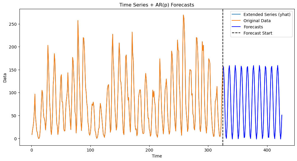
The predictions above are perfectly sinusoidal. Because the cycles for the sunspots data are irregular and can have different periods, there is a danger that these perfectly sinusoidal predictions can get out of phase sometimes leading to loss of prediction accuracy.
Below, we simulate datasets using the Yule model.
#Simulating from the Yule Model:
rng = np.random.default_rng(seed = 42)
sighat = np.sqrt(np.mean(yulemod.resid ** 2))
print(sighat)
fig, axes = plt.subplots(3, 3, figsize = (12, 6))
axes = axes.flatten()
for j in range(9):
ysim = y.copy()
for i in range(2, n):
err = rng.normal(loc = 0, scale = sighat, size = 1)
ysim[i] = yulemod.params[0] + yulemod.params[1] * ysim[i-1] - ysim[i-2] + err[0]
axes[j].plot(ysim)
plt.show()27.77831798002467
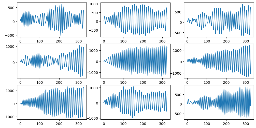
These datasets are quite smooth. This shows that the two “sinusoid + noise” models described in lecture are fundamentally different.
AR(2) Model
Now we apply the AR(2) model to the sunspots dataset.
sunspots = pd.read_csv('SN_y_tot_V2.0.csv', header = None, sep = ';')
y = sunspots.iloc[:,1].values
n = len(y)
plt.figure(figsize = (12, 6))
plt.plot(y)
plt.show()p = 2 #this is the order of the AR model
n = len(y)
print(n)325
yreg = y[p:] #these are the response values in the autoregression
Xmat = np.ones((n-p, 1)) #this will be the design matrix (X) in the autoregression
for j in range(1, p+1):
col = y[p-j : n-j].reshape(-1, 1)
Xmat = np.column_stack([Xmat, col])armod = sm.OLS(yreg, Xmat).fit()
print(armod.params)
print(armod.summary())
sighat = np.sqrt(np.mean(armod.resid ** 2))
print(sighat)[24.45610705 1.38803272 -0.69646032]
OLS Regression Results
==============================================================================
Dep. Variable: y R-squared: 0.829
Model: OLS Adj. R-squared: 0.828
Method: Least Squares F-statistic: 774.7
Date: Thu, 13 Mar 2025 Prob (F-statistic): 2.25e-123
Time: 23:57:29 Log-Likelihood: -1505.5
No. Observations: 323 AIC: 3017.
Df Residuals: 320 BIC: 3028.
Df Model: 2
Covariance Type: nonrobust
==============================================================================
coef std err t P>|t| [0.025 0.975]
------------------------------------------------------------------------------
const 24.4561 2.384 10.260 0.000 19.767 29.146
x1 1.3880 0.040 34.524 0.000 1.309 1.467
x2 -0.6965 0.040 -17.342 0.000 -0.775 -0.617
==============================================================================
Omnibus: 33.173 Durbin-Watson: 2.200
Prob(Omnibus): 0.000 Jarque-Bera (JB): 50.565
Skew: 0.663 Prob(JB): 1.05e-11
Kurtosis: 4.414 Cond. No. 231.
==============================================================================
Notes:
[1] Standard Errors assume that the covariance matrix of the errors is correctly specified.
25.588082517109108
#Simulations from the fitted AR(2) model:
fig, axes = plt.subplots(3, 3, figsize = (12, 6))
axes = axes.flatten()
for j in range(9):
ysim = y.copy()
for i in range(2, n):
err = rng.normal(loc = 0, scale = sighat, size = 1)
ysim[i] = armod.params[0] + armod.params[1] * ysim[i-1] + armod.params[2] * ysim[i-2] + err[0]
axes[j].plot(ysim)
plt.show()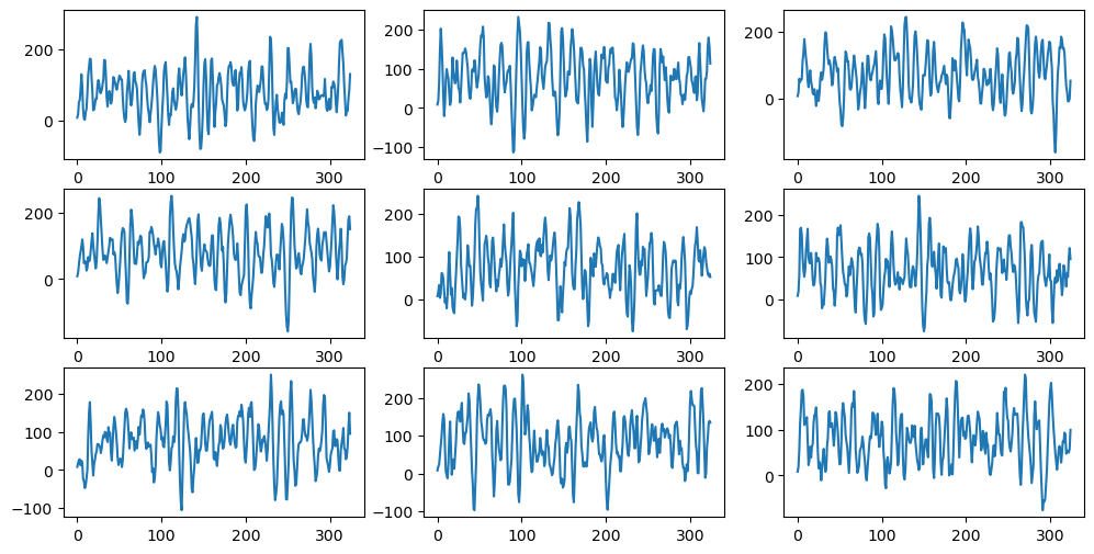
These datasets are still smooth (much smoother than observations simulated from ).
Below, we obtain predictions using the AR(2) model.
#Generate k-step ahead forecasts:
k = 100
yhat = np.concatenate([y, np.full(k, -9999)]) #extend data by k placeholder values
for i in range(1, k+1):
ans = armod.params[0]
for j in range(1, p+1):
ans += armod.params[j] * yhat[n+i-j-1]
yhat[n+i-1] = ans
predvalues = yhat[n:]
#Plotting the series with forecasts:
plt.figure(figsize=(12, 6))
time_all = np.arange(1, n + k + 1)
plt.plot(time_all, yhat, label='Extended Series (yhat)', color='C0')
plt.plot(range(1, n + 1), y, label='Original Data', color='C1')
plt.plot(range(n + 1, n + k + 1), predvalues, label='Forecasts', color='blue')
plt.axvline(x=n, color='black', linestyle='--', label='Forecast Start')
#plt.axhline(y=np.mean(y), color='gray', linestyle=':', label='Mean of Original Data')
plt.xlabel('Time')
plt.ylabel('Data')
plt.title('Time Series + AR(p) Forecasts')
plt.legend()
plt.show()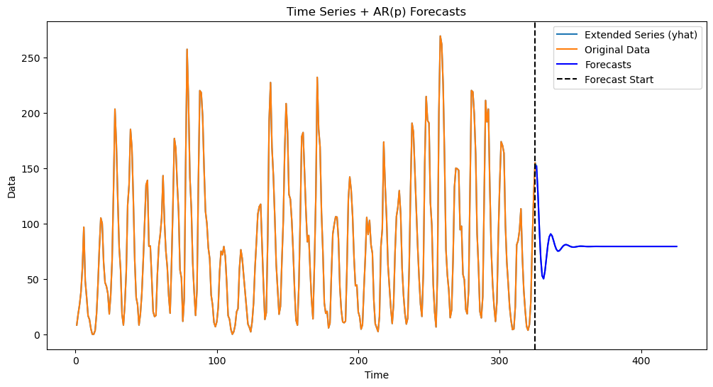
The predictions above are quite different from those obtained from the Yule model. The predictions actually are given be a damped sinusoid (as we shall see in the coming lectures). The predictions become flat after a few time points. When the cycles become irregular with varying periods, constant predictors might do well compared to sinusoidal predictors which may go out of phase at some places.